Working with Raster Data
In this exerciser we will learn following raster processing techniques with R:
R-Packages
- rgdal: Bindings for the Geospatial Data Abstraction Library
- raster: Geographic Data Analysis and Modeling
- RColorBrewer: ColorBrewer Palettes (making customize color palettes)
- classInt: Choose Uni variate Class Intervals
Load R packages
library (rgdal)           # Geospatial Data Abstraction Library
library (raster)          # raster data
library(classInt)     # for class interval
library(RColorBrewer)   # for customize colour palettes
library(gridExtra)    # plotting
library(spatialEco)   # Curveture analysis
Load Data
We will use elevation data (5 km x 5 km) of four states of great plain region of USA (GP_ELEV.tif) and data set could be available for download from here
# Define data folder
dataFolder<-"D://Dropbox//Spatial Data Analysis and Processing in R//DATA_07//DATA_07//"
Load raster
ELEV.GP<-raster(paste0(dataFolder,"GP_ELEV.tif"))Basic Raster Operation
Check projection system
ELEV.GP@crs## CRS arguments:
## +proj=aea +lat_1=29.5 +lat_2=45.5 +lat_0=23 +lon_0=-96 +x_0=0
## +y_0=0 +ellps=GRS80 +towgs84=0,0,0,0,0,0,0 +units=m +no_defsCheck raster attribute
ELEV.GP## class : RasterLayer
## dimensions : 310, 275, 85250 (nrow, ncol, ncell)
## resolution : 5000, 5000 (x, y)
## extent : -1250285, 124715, 988795, 2538795 (xmin, xmax, ymin, ymax)
## crs : +proj=aea +lat_1=29.5 +lat_2=45.5 +lat_0=23 +lon_0=-96 +x_0=0 +y_0=0 +ellps=GRS80 +towgs84=0,0,0,0,0,0,0 +units=m +no_defs
## source : D:/Dropbox/Spatial Data Analysis and Processing in R/DATA_07/DATA_07/GP_ELEV.tif
## names : GP_ELEV
## values : 224.4348, 3828.2 (min, max)- Nrow, Ncol: the number of rows and columns in the data (imagine a spreadsheet or a matrix).
- Ncells: the total number of pixels or cells that make up the raster.
- Resolution: the size of each pixel (deg decimal).
- Extent: the spatial extent of the raster. This value will be in the same coordinate units as the coordinate reference system of the raster.
- Coord ref: the coordinate reference system string for the raster. This raster is in Geographical Coordinate system with a datum of WGS 84.
Raster extent
extent(ELEV.GP)## class : Extent
## xmin : -1250285
## xmax : 124715
## ymin : 988795
## ymax : 2538795Raster statistics
R allow you to calculate some basic statistics of raster data. We can use summary function to get some statistics of raster layer.
summary(ELEV.GP)## GP_ELEV
## Min. 224.4348
## 1st Qu. 1207.6884
## Median 1633.6725
## 3rd Qu. 2160.3500
## Max. 3828.2000
## NA's 42766.0000Histogram of raster
R-base function hist is also useful to know frequency of raster values
HISTO.GP<-hist(ELEV.GP,
     breaks=6,
     col= "purple",                                              # color of histogram
     main="Distribution of Elevation values with 5 breaks",     # tittle of the plot
     xlab= "Elevation (m)",                                     # x-axis name
     ylab = "Number of Pixels")                                 # y-axis name
box()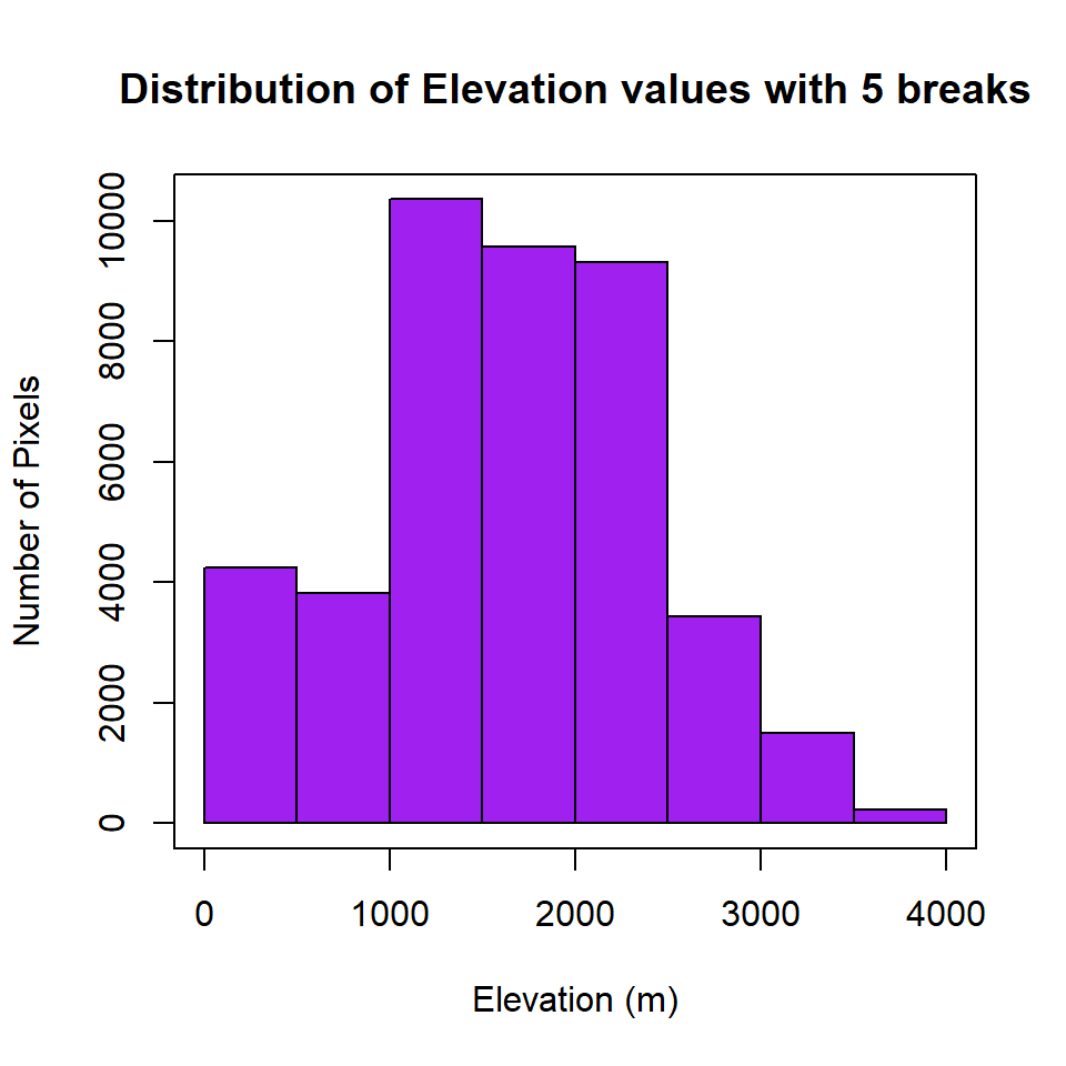
Plot raster
plot(ELEV.GP, main="Albers Equal Area Conic")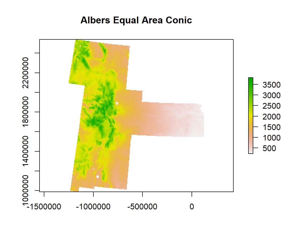
Clipping
Now will clip this DEM with extent of CO state shape file. Before clipping, you have to make sure both raster and vector data are in same projection systems.
# Load CO state shape file
CO.STATE<-shapefile(paste0(dataFolder,"CO_STATE_BD.shp"))
proj4string(CO.STATE)
## [1] "+proj=aea +lat_1=29.5 +lat_2=45.5 +lat_0=23 +lon_0=-96 +x_0=0 +y_0=0 +datum=NAD83 +units=m +no_defs +ellps=GRS80 +towgs84=0,0,0"In R, clipping of a raster is two steps procedure, first you have to apply crop() function & then mask functions of raster package. Crop returns a geographic subset of an object as specified by an extent object (or object from which an extent object can be extracted/created). mask Create a new Raster object that has the same values as input raster.
ELEV.CO<- crop(ELEV.GP, extent(CO.STATE))
ELEV.CO <-raster::mask(ELEV.CO, CO.STATE)
writeRaster(ELEV.CO, paste0(dataFolder,"CO_ELEV.tiff"),"GTiff",overwrite=TRUE)
Plot Clip DEM
plot(ELEV.CO, main= "5 km x 5 Km DEM of CO State")
plot(CO.STATE, add=TRUE)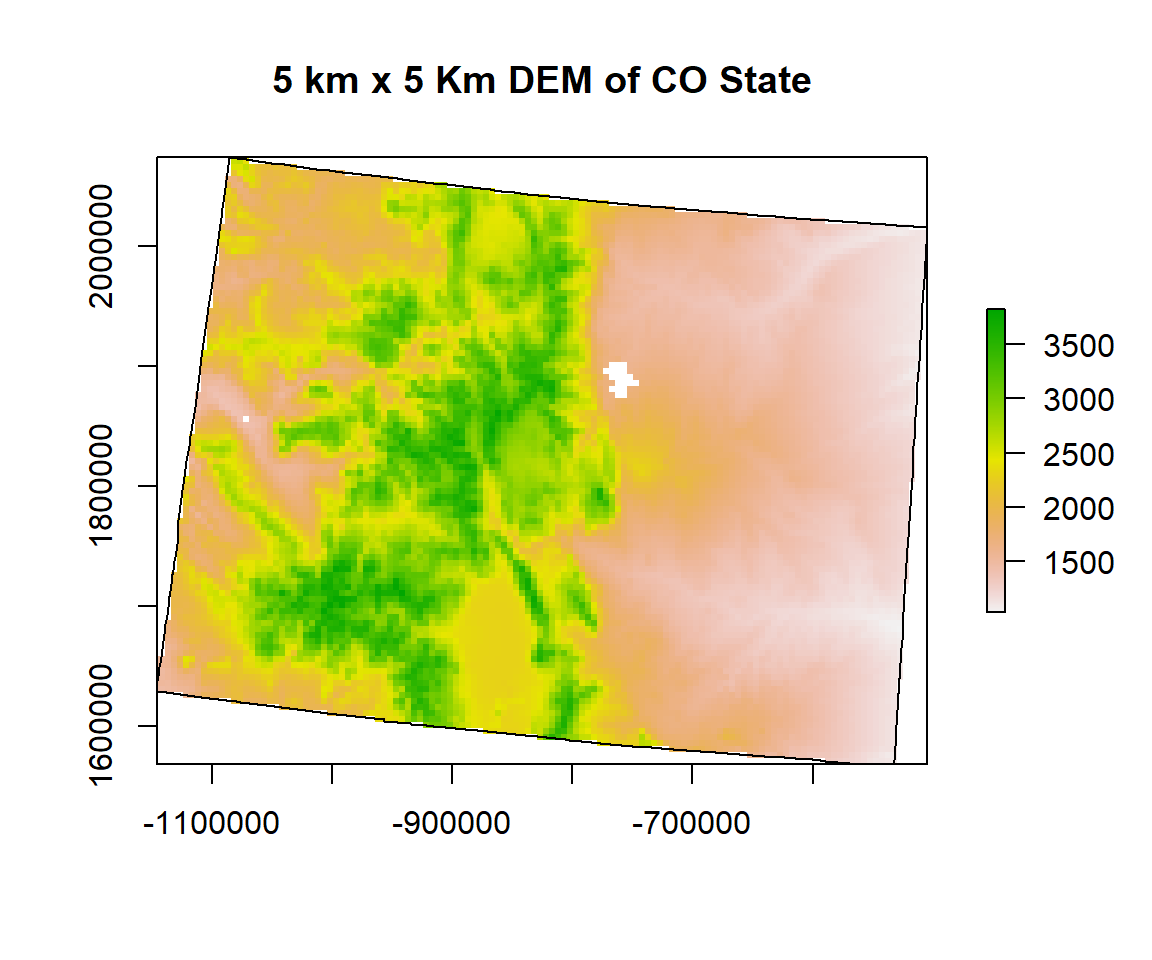
Reclassification
Histogram
Before reclassification, we create a histogram with 4 breaks, of ELEV.CO raster
HISTO.CO<-hist(ELEV.CO,
     breaks=3,
     col= "purple",                                             # color of histogram
     main="Distribution of Elevation values with 4 breaks",     # tittle of the plot
     xlab= "Elevation (m)",                                     # x-axis name
     ylab = "Number of Pixels")                                 # y-axis name
box()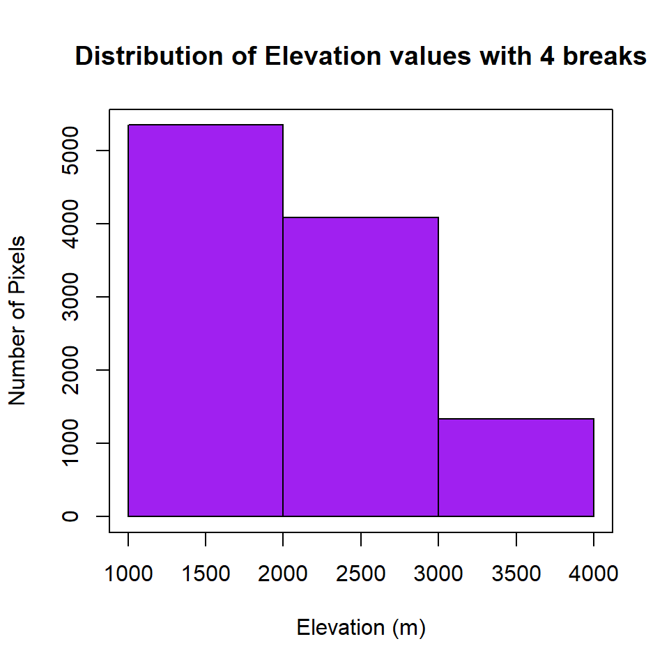
Now, you can check where are breaks and how many pixels in each category, and use these breaks to plot a raster layer
HISTO.CO$breaks## [1] 1000 2000 3000 4000HISTO.CO$counts## [1] 5347 4083 1335# plot using the histogram breaks.
plot(ELEV.CO,
breaks = c(1000, 2000, 3000, 4000),
col = terrain.colors(5),
main="DEM ")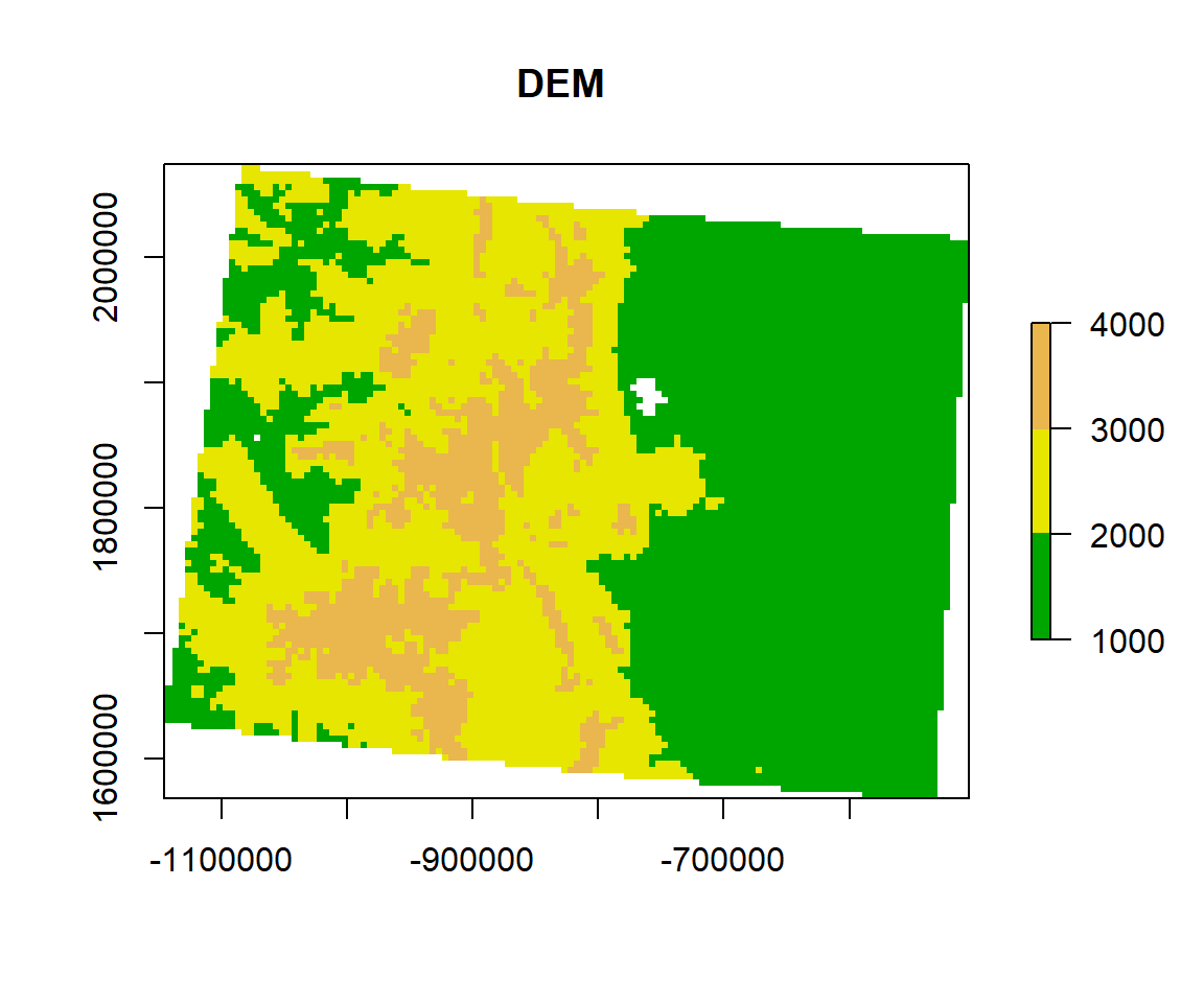
We will use breaks of histogram to reclassify the DEM raster. First, you have to create classification matrix
- Class 1: 1000 - 2000 m (low elevation)
- Class 2: 2000 - 3000 m (medium elevation)
- Class 3: 3000 - 4000 (Inf) m (high elevation)
# Create a dataframe
reclass_df <- c(1000, 2000, 1,
                2000, 3000, 2,
                3000, Inf, 3)
reclass_df
## [1] 1000 2000 1 2000 3000 2 3000 Inf 3Next, you have to reshape the data frame to matrix using matrix function
reclass_m <- matrix(reclass_df,
                ncol = 3,
                byrow = TRUE)
reclass_m
## [,1] [,2] [,3]
## [1,] 1000 2000 1
## [2,] 2000 3000 2
## [3,] 3000 Inf 3Now you have to apply reclassify() function of raster package using re-class_m object.
ELEV.CO.reclass <- reclassify(ELEV.CO,
                     reclass_m)
You can view the distribution of pixels assigned to each class using the bar-plot().
barplot(ELEV.CO.reclass,
        main = "Number of pixels in each class")
box()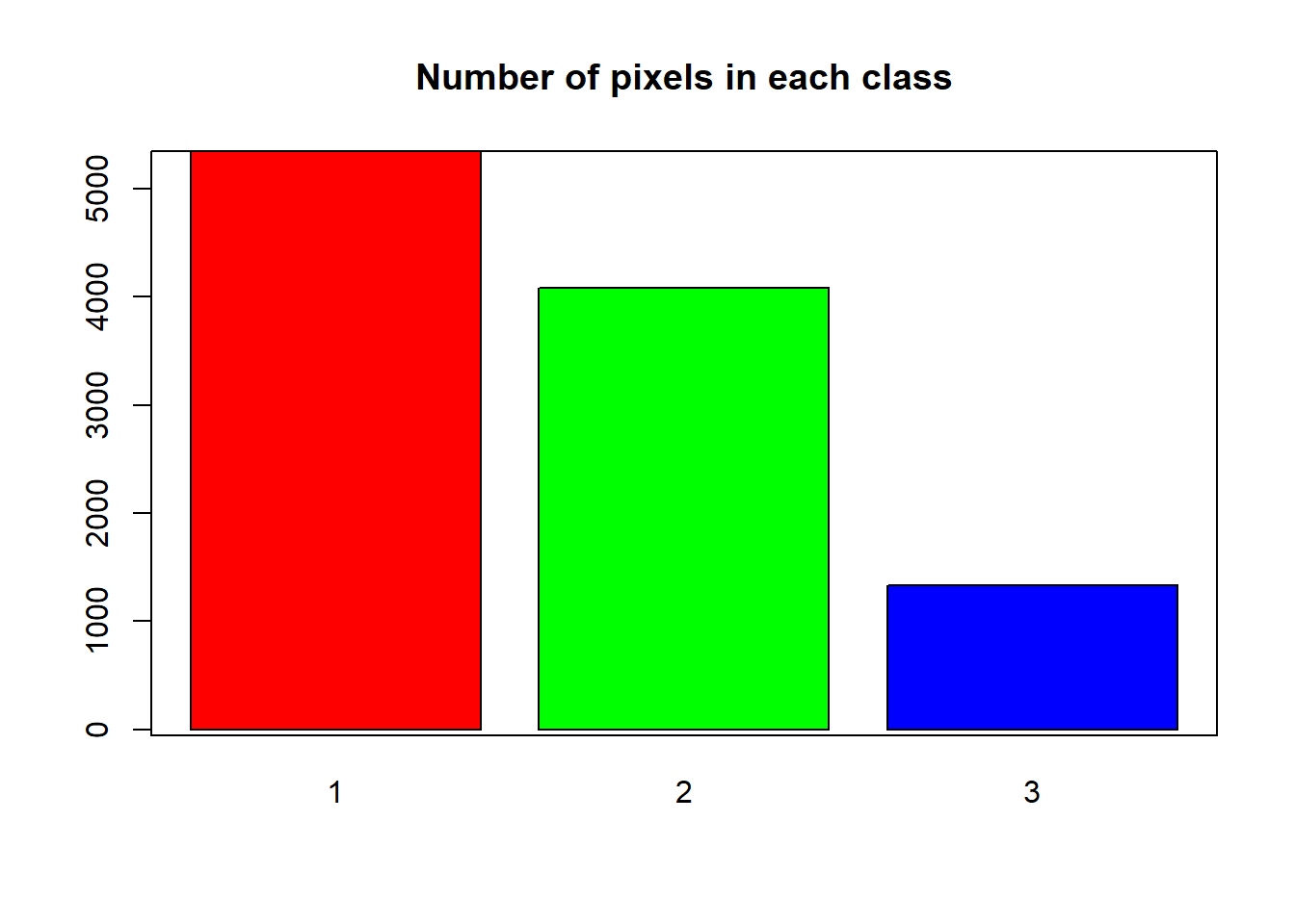
Now we plot the reclassified raster using plot function with a nice looking legend
plot(ELEV.CO.reclass,
     legend = FALSE,
     col = c("green", "blue", "red"), axes = FALSE,
     main = "Reclassified DEM")

legend("topright",
       legend = c("Low", "Medium", "High"),
       fill = c("green", "blue", "red"),
       border = FALSE,
       bty = "n") # turn off legend border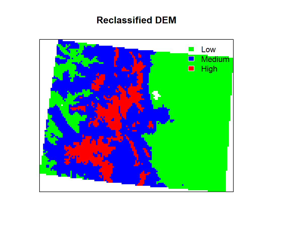
Quantile
Sometimes quantile function is us full to the distribution of raster values
quantile(ELEV.CO) # default 5 quantile## 0% 25% 50% 75% 100%
## 1032.333 1490.708 2006.680 2608.840 3828.200quantile(ELEV.CO, prob=seq(0,1,0.1)) # 10 quantile## 0% 10% 20% 30% 40% 50% 60% 70%
## 1032.333 1280.194 1418.156 1567.555 1770.616 2006.680 2267.440 2480.909
## 80% 90% 100%
## 2756.125 3089.469 3828.200Define quantile breaks
If you want create a raster map using the quantile, you fave to use classInt package. The classIntervals function is create a custom breaks of raster values using different styles (such as “fixed”, “sd”, “equal”, “pretty”, “quantile”, “kmeans”, “hclust”, “bclust”, “fisher”, & “jenks”). For details, please see help, just type ?classIntervals in R console
First, we have to convert raster to vector using values function. Then, you have to create a object with a quantile interval applying classIntervals function to vector data.
value.vector <- values(ELEV.CO)
value.vector <- value.vector[value.vector != 0]
at = round(classIntervals(value.vector, n = 10, style = "quantile")$brks, 0) # 10 quantile
at
## [1] 1032 1280 1418 1568 1771 2007 2267 2481 2756 3089 3828Now, we plot the DEM raster using the this custom break. We will use sppot function from sp package to plot raster data with state boundary shape file. Before that we will create a custom color palette using colorRampPalette of RColorBrewer.
rgb.palette <- colorRampPalette(c("lightblue","blue","green","yellow","red"),
space = "rgb")
polys<- list("sp.lines", as(CO.STATE, "SpatialLines"), col="grey", lty=1)  # CO state boundary
spplot(ELEV.CO, main = "Quantile of DEM (m)",
   at=at,sp.layout=list(polys),
   par.settings=list(axis.line=list(col="darkgrey",lwd=1)),
   colorkey=list(space="right",height=1, width=1.3,at=1:11,labels=list(cex=1.0,at=1:11,
   labels=c("1032","1280","1418","1568","1771","2007","2267","2481","2756","3089","3828"))),
   col.regions=rgb.palette(100))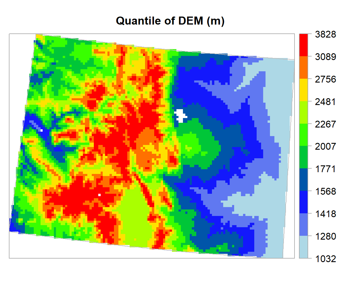
Focal Statistics
Focal statistics calculate for each input cell location a statistic (mean, sum etc) of the values within a specified neighborhood around it. Conceptually, on execution, the algorithm visits each cell in the raster and calculates the specified statistic with the identified neighborhood. The cell for which the statistic is being calculated is referred to as the processing cell. The value of the processing cell, as well as all the cell values in the identified neighborhood, is included in the neighborhood statistics calculation. The neighborhoods can overlap so that cells in one neighborhood may also be included in the neighborhood of another processing cell. (Source:http://resources.arcgis.com/EN/HELP/MAIN/10.2/index.html#/How_Focal_Statistics_works/009z000000r7000000/)
To illustrate the neighborhood processing for Focal Statistics calculating a Sum statistic, consider the processing cell with a value of 5 in the following diagram. A rectangular 3 by 3 cell neighborhood shape is specified. The sum of the values of the neighboring cells (3 + 2 + 3 + 4 + 2 + 1 + 4 = 19) plus the value of the processing cell (5) equals 24 (19 + 5 = 24). So a value of 24 is given to the cell in the output raster in the same location as the processing cell in the input raster.

Focal Statistics(Source: http://resources.arcgis.com/EN/HELP/MAIN/10.2/index.html#/How_Focal_Statistics_works/009z000000r7000000/)
The above figure demonstrates how the calculations are performed on a single cell in the input raster. In the following diagram, the results for all the input cells are shown. The cells highlighted in yellow identify the same processing cell and neighborhood as in the example above.
We will calculate focal mean of each cell of DEM data using focal() function of raster package.
focal.sum<- focal(ELEV.CO,
    w=matrix(1/9,nrow=3,ncol=3),    # matrix of weights for 3 x 3
    fun=sum)
spplot(focal.sum, main="Focal Sum of DEM (m)")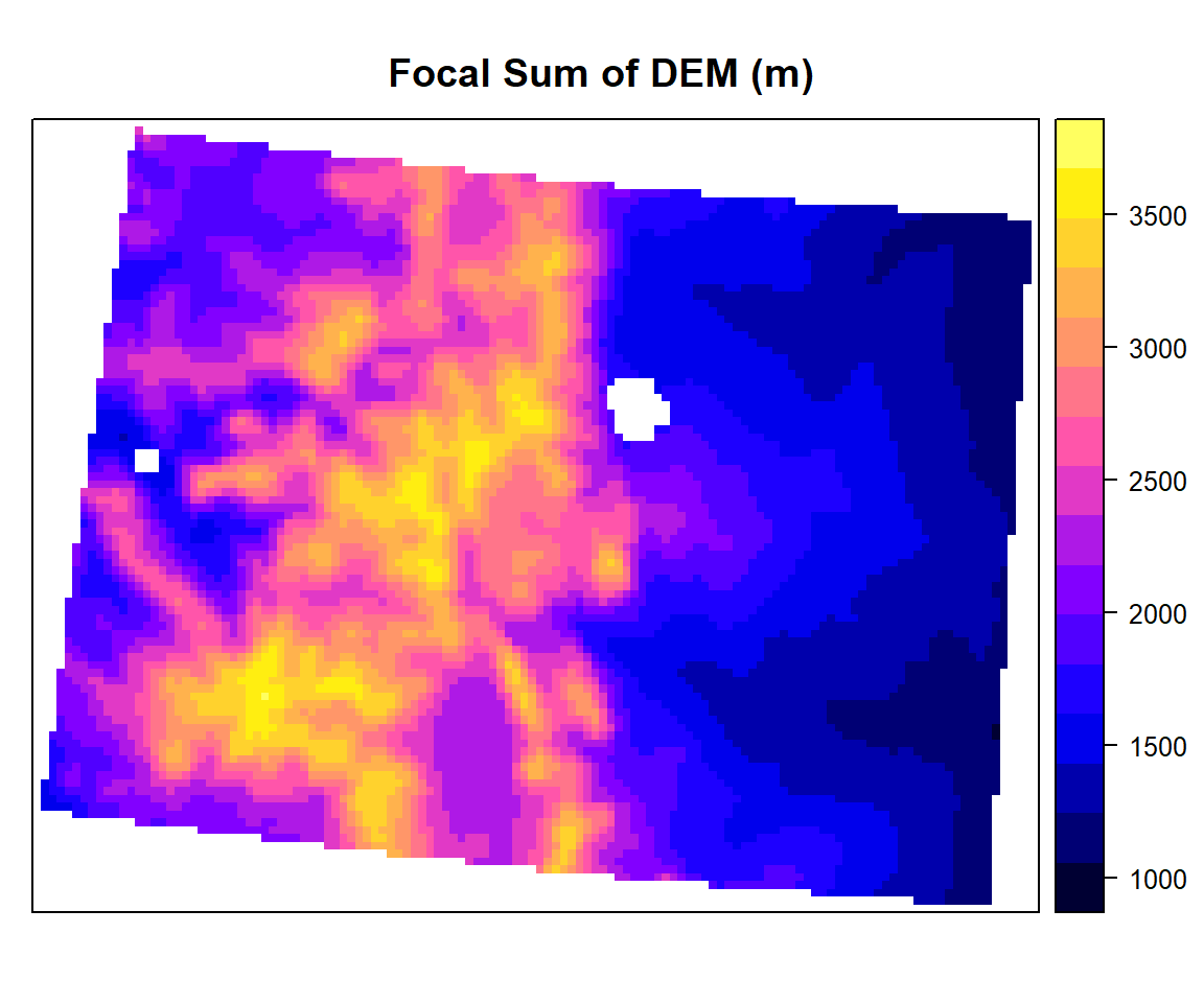
focal.mean<- focal(ELEV.CO,
    w=matrix(1/9,nrow=3,ncol=3),    # matrix of weights for 3 x 3
    fun=mean)
spplot(focal.mean,main="Focal Mean of DEM (m)")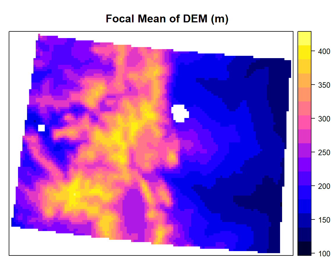
Raster Algebra
Raster algebra in R is a set-based algebra for manipulating a raster object more raster layers (“maps”) of similar dimensions to produce a new raster layer (map) using algebraic operations. It includes the normal algebraic operators such as +, -, *, /, logical operators such as >, >=, <, ==, ! and functions like abs, round, ceiling, floor, trunc, sqrt, log, log10, exp, cos, sin, atan, tan, max, min, range, prod, sum, any, all.
A simple sample of raster algebra in R is to convert unit of DEM raster from meter to feet (1 m = 3.28084 feet)
dem.feet<-ELEV.CO*3.28084plot(dem.feet, main= "DEM (feet)")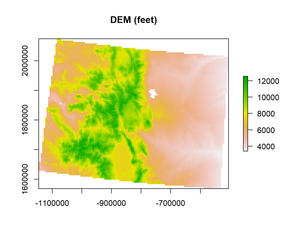
dem.feet.1000<-dem.feet/1000
plot(dem.feet.1000, main = "DEM (feet x 1000)")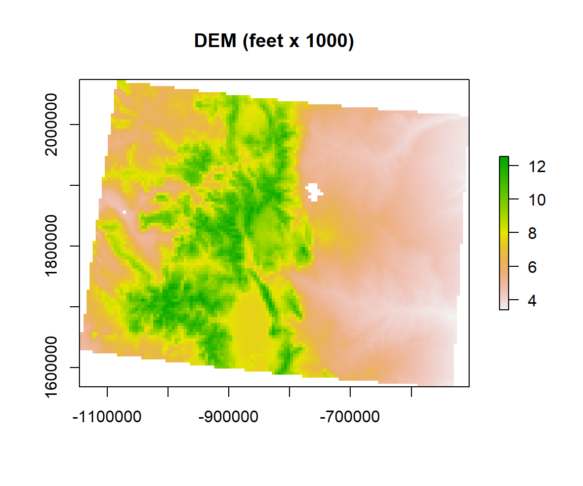
Aggregation
Aggregate a Raster object to create a new Raster-layer with a lower resolution (larger cells). Aggregation groups rectangular areas to create larger cells. The value for the resulting cells is computed with a user-specified function. First, we will create 10 km x 10 km raster (mean & standard deviation) from 5 km x 5 kg raster using aggregate function of raster package. If aggregate function does not work, remove “mean” or “sd” objects if you have created before.
#rm(mean)
#rm(sd)
mean.DEM<-aggregate(ELEV.CO, fact=2, fun=mean)
sd.DEM<-aggregate(ELEV.CO, fact=2, fun=sd)
se.DEM<-sd.DEM/sqrt(2)
mean.DEM
## class : RasterLayer
## dimensions : 51, 64, 3264 (nrow, ncol, ncell)
## resolution : 10000, 10000 (x, y)
## extent : -1145285, -505285, 1563795, 2073795 (xmin, xmax, ymin, ymax)
## crs : +proj=aea +lat_1=29.5 +lat_2=45.5 +lat_0=23 +lon_0=-96 +x_0=0 +y_0=0 +ellps=GRS80 +towgs84=0,0,0,0,0,0,0 +units=m +no_defs
## source : memory
## names : GP_ELEV
## values : 1052.791, 3692.687 (min, max)p1<-spplot(mean.DEM, main="Mean (10 km x 10 km) of DEM (m)")
p2<-spplot(sd.DEM, main="SD of DEM (m)")
p3<-spplot(se.DEM, main="SE of DEM (m)")
grid.arrange(p1, p2, p3, ncol=3)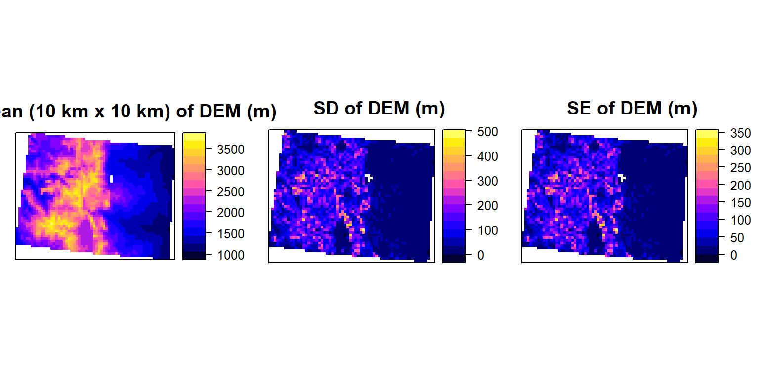
Resample
Re-sample transfers values between non matching Raster in in terms of origin and resolution. We will re-sample 10 km raster to 5 km raster again using ELEV.CO ( 5 km). We will use resample function. Here two methods available: bilinear for bilinear interpolation, or **ngb* for using the nearest neighbor. First argument is a raster object to be re-sampled and second argument is raster object with parameters that first raster should be re-sampled to.
dem.5km<-resample(mean.DEM, ELEV.CO, method='bilinear') #
dem.5km
## class : RasterLayer
## dimensions : 101, 128, 12928 (nrow, ncol, ncell)
## resolution : 5000, 5000 (x, y)
## extent : -1145285, -505285, 1568795, 2073795 (xmin, xmax, ymin, ymax)
## crs : +proj=aea +lat_1=29.5 +lat_2=45.5 +lat_0=23 +lon_0=-96 +x_0=0 +y_0=0 +ellps=GRS80 +towgs84=0,0,0,0,0,0,0 +units=m +no_defs
## source : memory
## names : GP_ELEV
## values : 1045.513, 3630.237 (min, max)spplot(dem.5km, main="Resampled DEM - 5 x 5 km")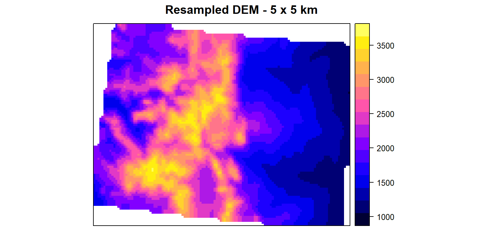
Mosaic
We will use merge() function to mosaic all raster ./DEM.GP folder to create a seamless raster of great plain
DEM.input <- list.files(path= paste0(dataFolder,".//DEM_GP"),pattern=".tif$",full.names=T)
DEM.input
## [1] "D://Dropbox//Spatial Data Analysis and Processing in R//DATA_07//DATA_07//.//DEM_GP/CO_ELEV.tif"
## [2] "D://Dropbox//Spatial Data Analysis and Processing in R//DATA_07//DATA_07//.//DEM_GP/KS_ELEV.tif"
## [3] "D://Dropbox//Spatial Data Analysis and Processing in R//DATA_07//DATA_07//.//DEM_GP/NM_ELEV.tif"
## [4] "D://Dropbox//Spatial Data Analysis and Processing in R//DATA_07//DATA_07//.//DEM_GP/WY_ELEV.tif"r <- lapply(DEM.input, raster)
r1<-do.call(merge, c(r, tolerance = 1))plot(r1, main="Mosaic DEM (m)")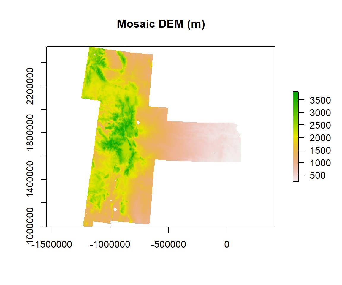
Convert Raster to Point Data
For convert raster data to spatial point data frame, we will use rasterToPoints() function and then we will apply as.data.frame() function to convert a regular data frame
SPDF <- rasterToPoints(ELEV.CO)
str(SPDF)
## num [1:10765, 1:3] -1082785 -1077785 -1072785 -1082785 -1077785 ...
## - attr(*, "dimnames")=List of 2
## ..$ : NULL
## ..$ : chr [1:3] "x" "y" "GP_ELEV"df<-as.data.frame(SPDF)
head(df)## x y GP_ELEV
## 1 -1082785 2071295 2568.92
## 2 -1077785 2071295 2610.72
## 3 -1072785 2071295 2393.16
## 4 -1082785 2066295 2498.28
## 5 -1077785 2066295 2481.25
## 6 -1072785 2066295 2610.20write.csv(df, paste0(dataFolder,"GP_ElEV.csv", row.names = F))Convert Point Data to Raster
First, we will convert df to a SpatialPointsDataFrame, then we will use rasterFromXYZ to convert point data frame to raster. Finally, we will define CRS to Albers Equal Area Conic
x<-SpatialPointsDataFrame(df[, c("x", "y")], data = df)
DEM <- rasterFromXYZ(as.data.frame(x)[, c("x", "y", "GP_ELEV")])
usa_albers = CRS("+proj=aea +lat_1=20 +lat_2=60 +lat_0=40 +lon_0=-96 +x_0=0 +y_0=0 +datum=NAD83 +units=m +no_defs")
proj4string(DEM) = usa_albers
spplot(DEM)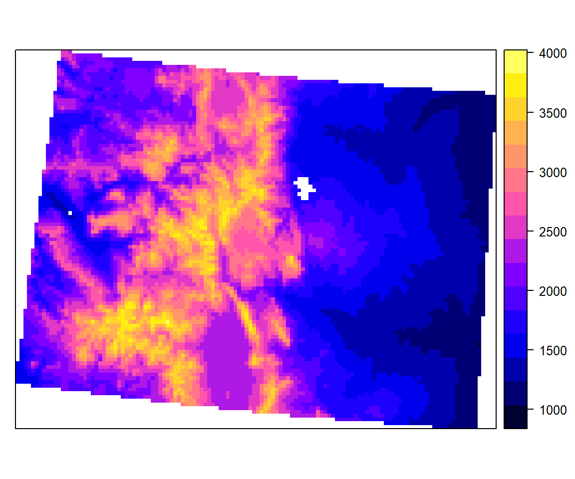
Raster Stack and Raster Brick
You can use High-level functions to manipulate multiple raster after creating create raster stack (collection of raster layers) using stack() or brick() functions of raster raster package. The stack() and bricck() functions can both store multiple layers. However, how they store each layers is different. The layers in a in stack() are stored as links to raster data that is located somewhere on our computer. A brick() contains all of the objects stored within the actual R object. brick() is more efficient and faster than stack(), We will use mean.DEM and sd.DEM raster to create standard error map.
s<-stack(mean.DEM,sd.DEM, se.DEM) # stack
names(s)<-c("Mean", "SD","SE")  # rename the layers
s
## class : RasterStack
## dimensions : 51, 64, 3264, 3 (nrow, ncol, ncell, nlayers)
## resolution : 10000, 10000 (x, y)
## extent : -1145285, -505285, 1563795, 2073795 (xmin, xmax, ymin, ymax)
## crs : +proj=aea +lat_1=29.5 +lat_2=45.5 +lat_0=23 +lon_0=-96 +x_0=0 +y_0=0 +ellps=GRS80 +towgs84=0,0,0,0,0,0,0 +units=m +no_defs
## names : Mean, SD, SE
## min values : 1052.791, 0.000, 0.000
## max values : 3692.6873, 470.5111, 332.7016spplot(s)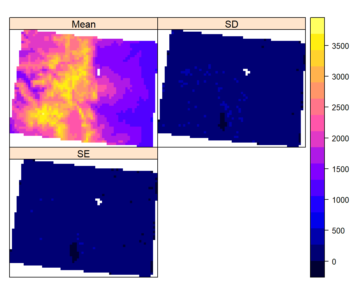
Digital Terrain Modeling
Terrain analysis or land surface analysis is a process that describes terrain, for example it’s roughness, altitude, etc., quantitatively. Such analysis can be very useful in assessing land suitability for agriculture, construction, roads, or in designing irrigation schemes, and other land use features.
Slope
The slope is an incline, or steepness, of a surface. The slope can be measured in degrees from horizontal (0-90), or percent slope (which is the rise divided by the run, multiplied by 100). A slope of 30 and 45 degrees equals 58 and 100 percent slope, respectively. As the slope angle approaches vertical (90 degrees), the percent slope approaches infinity. The slope for a cell in a raster is the steepest slope of a plane defined by the cell and its eight surrounding neighbors. (Source: ESRI online GIS Dictionary).

Slope(Source: http://resources.arcgis.com/EN/HELP/MAIN/10.2/index.html#/How_Focal_Statistics_works/009z000000r7000000/)
We will use terrain() function from raster package to create raster slope.
SLOPE <- terrain(ELEV.CO,           # raster DEM
    opt="slope",                        # Slope function
    unit='degrees')                 # unit degree
plot(SLOPE,
col = rainbow(16), main= "Slope (degree)")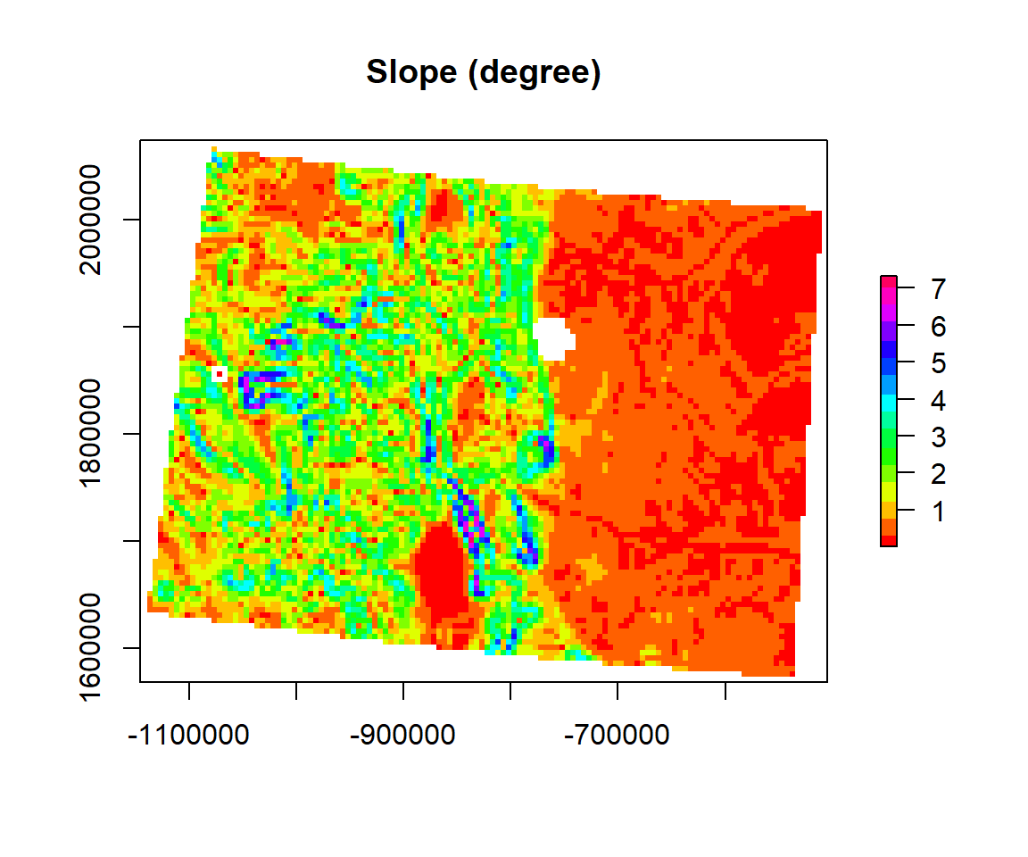
Aspect
The compass direction that a slope faces is most commonly measured from degrees north. The Aspect command provides a 32-bit float raster that ranges from 0° and 360°. This represents the azimuth (the angular distance from the north to south point of the horizon that can be transversed by a vertical circle that intersects the horizon, which represents the direction of an object from the observer) that slopes are facing. In other words, 0° means that the slope is facing North, 90° indicates East, 180° indicates a Southward facing, and 270° is to the west. This however requires that the top of your input raster is north oriented, as most are. Values found in between these ranges assume a mixture of cardinal directions, ex. 250 indicates a hillside with a Southeast facing aspect. The aspect value -9999 is generally used as the ‘nodata’ value to indicate use of an undefined aspect in areas lacking variation in topography, with slope=0. You can also make use of the legend to indicate the appropriate aspect for each hillside in your study area. The legend permits you to identify North (~ 0 or 360 degrees), South (~ 180 degrees), East (~270 degrees) or West (~90 degrees) facing slopes).

Aspect(Source: http://resources.arcgis.com/EN/HELP/MAIN/10.2/index.html#/How_Focal_Statistics_works/009z000000r7000000/)
ASPECT <- terrain(ELEV.CO,        #  raster DEM
    opt="aspect",                       #  aspect function
    unit='degrees')                   #  unit degree
plot(ASPECT,
col = rainbow(16), main= "Aspect (degree)")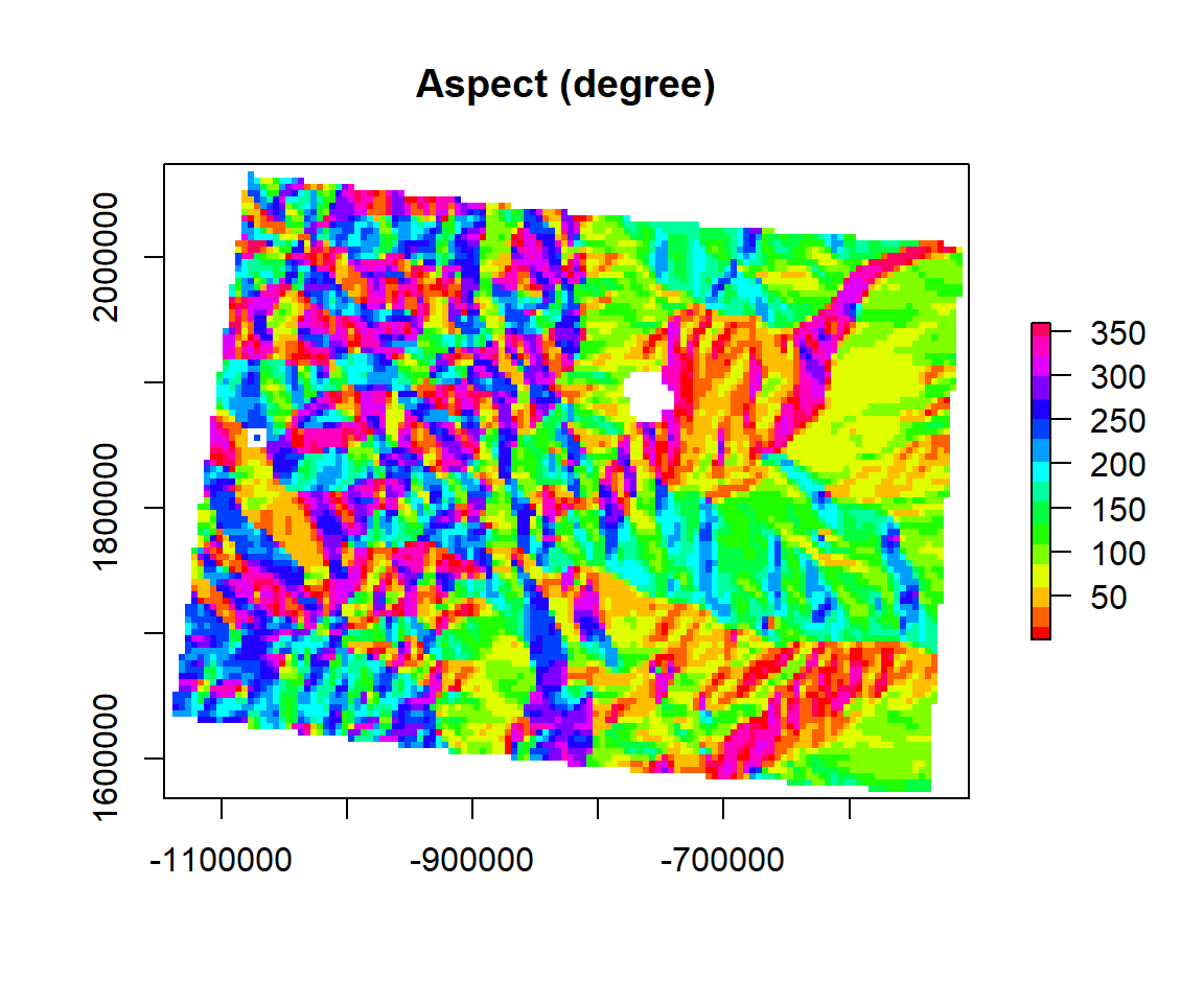
Hillshade

Hill Shade(Source: http://desktop.arcgis.com/en/arcmap/10.3/manage-data/raster-and-images/hillshade-function.htm)
We generate a hill shade layer from slope and aspect layers (both in degree). Slope and aspect can be computed with function terrain. A hill shade layer is often used as a backdrop on top of which another, semi-transparent, layer is drawn.
hill <- hillShade(SLOPE, ASPECT, 45, 250)
plot(hill, col=grey(0:100/100), legend=FALSE, main='Hillshade Map of CO')
plot(ELEV.CO, col=rainbow(50, alpha=0.35), add=TRUE)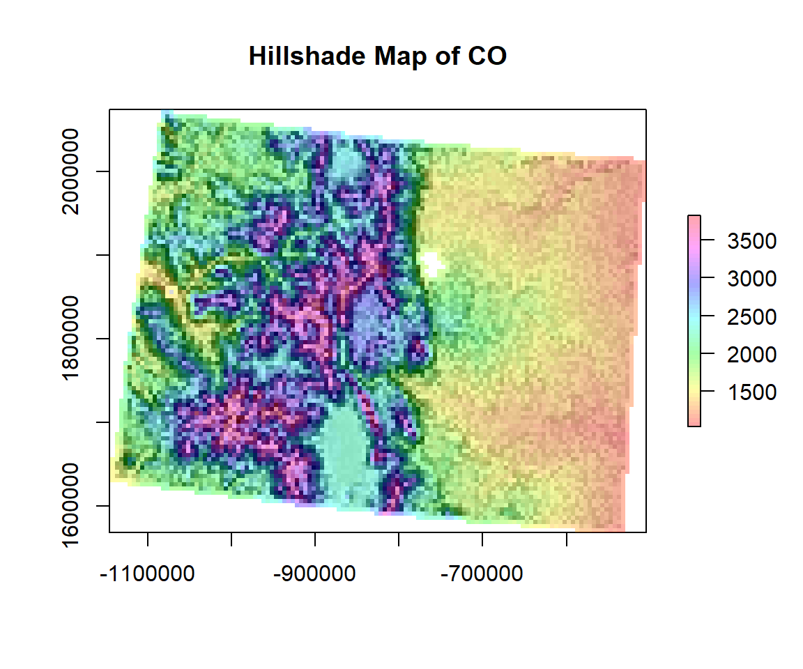
Terrain Ruggedness Index
TRI (Terrain Ruggedness Index) is the mean of the absolute differences between the value of a cell and the value of its 8 surrounding cells (the amount of elevation difference between adjacent cells of a DEM). This provides a relative measure of elevation changes between a specified grid cell and neighbors. The TRI is useful for analyzing what environments might be suited to particular crops or species which may be sensitive to particular sloped environments, or for assessing the potential flow of soil during erosion events, and so on.
TRI<- terrain(ELEV.CO,          #  raster DEM
    opt="TRI",                  #  TRI function
    unit='degrees')                 #  unit degree
plot(TRI,
main= "Terrain Ruggedness Index (TRI)",
col=rainbow(50))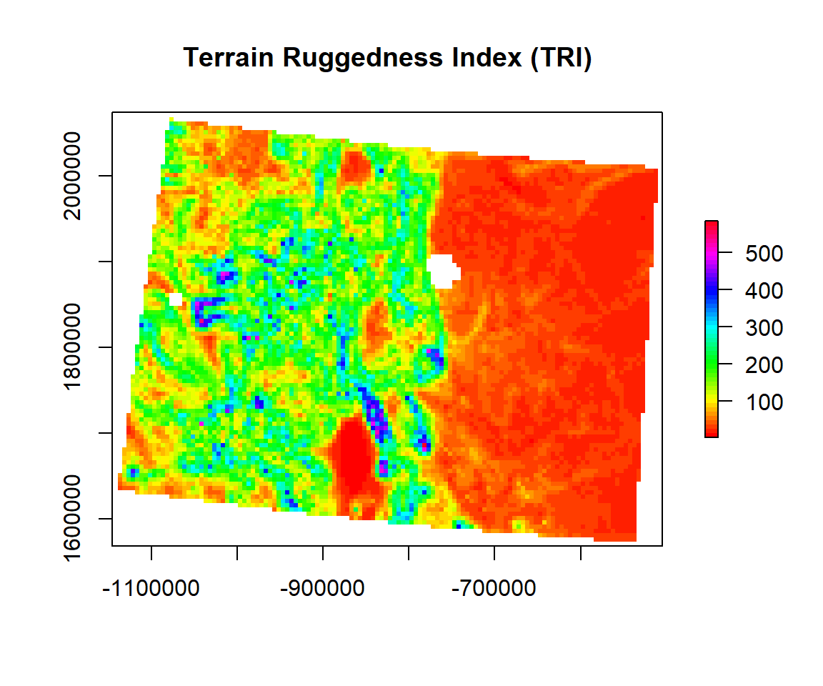
Topographic Position Index
TPI (Topographic Position Index) is the difference between the value of a cell and the mean value of its 8 surrounding cells.Positive TPI values represent locations that are higher than the average of their surroundings, as defined by the neighborhood (ridges). Negative TPI values represent locations that are lower than their surroundings (valleys). TPI values near zero are either flat areas (where the slope is near zero) or areas of constant slope. Topographic position is an inherent scale-dependent phenomenon.
TPI<- terrain(ELEV.CO,          #  raster DEM
    opt="TPI",                  #  TPI function
    unit='degrees')                 #  unit degree
plot(TPI,
main= "Topographic Position Index (TPI)",
col=rainbow(50))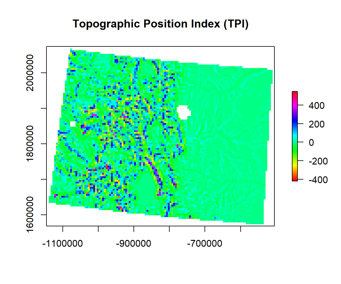
Roughness
Roughness is the difference between the maximum and the minimum value of a cell and its 8 surrounding cells.
ROUGH<- terrain(ELEV.CO,          # raster DEM
    opt="roughness",            # roughness function
    unit='degrees')                 # unit degree
plot(ROUGH,
main= "Roughness",
col=rainbow(50))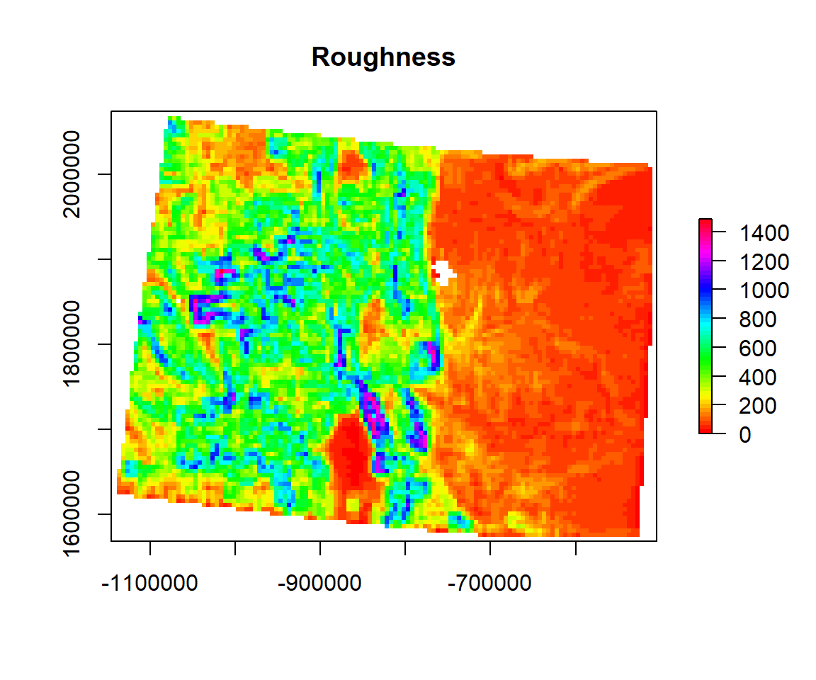
Curvature
Curvature is the change in the degree of slope for a given distance on that slope. It is a very helpful measure to understand the surface water flow through a landscape, and can be used in part to help design an irrigation scheme, for example. It is widely used by hydrological scientists. When interpreting data from a curve, any positive values indicate a convex (upward bulging) slope, while negative values correspond to a convex (downward facing) curve. The first is like a dinner bowl sanding correctly on a table, the latter is like a bowl that has been flipped over and is facing down. Any pixels observed that show positive curvature indicate the potential for liquid flow dispersal away from a central area, while and negative values indicate accumulation. In combination, convex and concave surfaces approximate actual topography.
A Plan curve is the measurement of the rate at which a horizontal curve changes. Positive and negative values respectively indicate divergence and convergence of a particular slope. Highlight a divergent slope, negative values a convergent slope.
A Profile curve is conversely a vertical measurement of the change of a slope. Positive values indicate convexity, while negative values represent concave profiles.

Hill Shade(Source: http://desktop.arcgis.com/en/arcmap/10.3/manage-data/raster-and-images/hillshade-function.htm)
In there is no package available yet for Curvature analysis in R. I have a function here. We will call this function using source(“curveture_function.R”), But when I run this, it shows error.
#source("curveture_function.R")
# profile<-curv(DEM, calc = "profile")
# plan<-curv(DEM, calc = "plan")
However, in spatialEco package allow to calculate McNab’s and Bolstad’s variants of the surface curvature (concavity/convexity) index (McNab 1993; Bolstad & Lillesand 1992; McNab 1989). The index is based on features that confine the view from the center of a 3x3 window. In the Bolstad equation, edge correction is addressed be dividing by the radius distance to the outermost cell (36.2m). We will use curveture function of spatialEco package.
# McNab curvature
m.crv <- curvature(ELEV.CO, s=5, type="mcnab")
# Bolstad curvature
b.crv <- curvature(ELEV.CO, s=5, type="bolstad")
p1<-spplot(m.crv, main="McNab curvature")
p2<-spplot(b.crv, main="Bolstad curvature")
grid.arrange(p1, p2, ncol=2)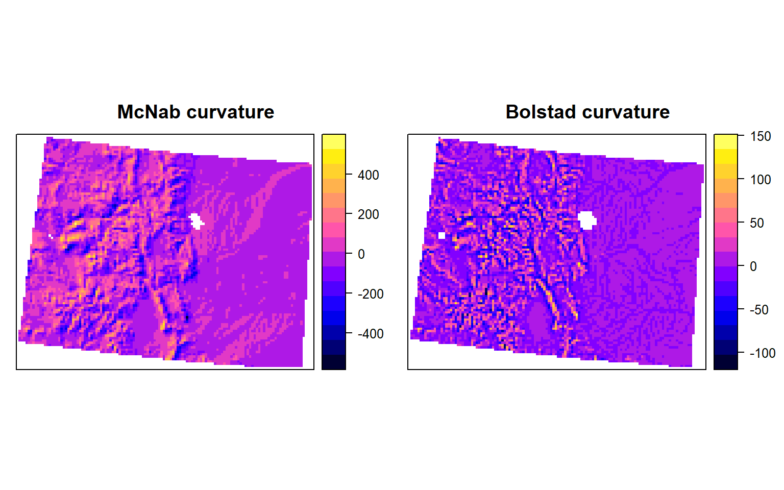
Flow Direction
The direction of the greatest drop in elevation (or the smallest rise if all neighbors are higher).
FLD<- terrain(ELEV.CO,          #  raster DEM
    opt="flowdir ",             # flow direction
    unit='degrees')                 # unit degree
plot(FLD,
main= "Flow Direction",
col=rainbow(50))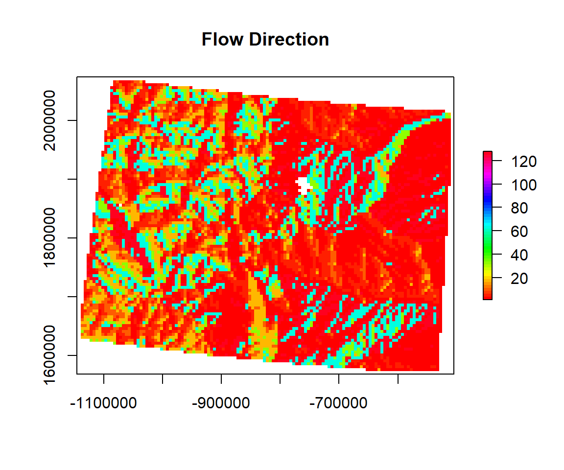
rm(list = ls())