Conditional Simulation for Spatial Uncertainty

This kriging prediction map smooth out local details of spatial distribution of the attribute under study, with small values being overestimated while large values are underestimated especially in area with low sampling density (Isaaks and Srivastava 1989). Conditional sequential Gaussian simulation (CSGS) techniques, unlike kriging, produce a better picture of reality and eliminate the unrealistic smoothing with focusing on the reproduction of global statistics or the semivariogram model in addition to honoring of original data values (Goovaerts 1997). The set of alternative realizations generated with CSGS provides a degree of uncertainty about the spatial prediction, which usually uses to draw reliable probability map of the variables under study (Goovaerts 1997). The CSGS is thus increasingly preferred to kriging for characterization of uncertainty for decision and risk analysis rather producing the best unbiased prediction of un-sampled location as is done with kriging (Deutsch and Journel 1998).

Load package:

library(plyr)
library(dplyr)
library(gstat)
library(raster)
library(rasterVis)
library(ggplot2)
library(car)
library(sp)
library(classInt)
library(RStoolbox)
library(gridExtra)

Load Data

The soil organic carbon data (train and test data set) that we have created before is available for download from here.

dataFolder<-"D:\\Dropbox\\Spatial Data Analysis and Processing in R\\DATA_08\\DATA_08\\"

state<-shapefile(paste0(dataFolder,"GP_STATE.shp"))
train<-read.csv(paste0(dataFolder,"train_data.csv"), header= TRUE) 
grid<-read.csv(paste0(dataFolder, "GP_prediction_grid_data.csv"), header= TRUE)
grid.xy<-grid[,1:3]

Data Transformation

Power Transform uses the maximum likelihood-like approach of Box and Cox (1964) to select a transformation of a univariate or multivariate response for normality. First we have to calculate appropriate transformation parameters using powerTransform() function of car package and then use this parameter to transform the data using bcPower() function.

powerTransform(train$SOC)

## Estimated transformation parameter 
## train$SOC 
## 0.2523339

train$SOC.bc<-bcPower(train$SOC, 0.2523339)

First. we have to define x & y variables as coordinates

coordinates(train) = ~x+y
coordinates(grid) = ~x+y

Variogram Modeling

# Variogram
v<-variogram(SOC.bc~ 1, data = train, cloud=F)
# Intial parameter set by eye esitmation
m<-vgm(1.5,"Exp",40000,0.5)
# least square fit
m.f<-fit.variogram(v, m)
m.f

##   model     psill    range
## 1   Nug 0.5165678     0.00
## 2   Exp 1.0816886 82374.23

Plot varigram and fitted model

#### Plot varigram and fitted model:
plot(v, pl=F, 
     model=m.f,
     col="black", 
     cex=0.9, 
     lwd=0.5,
     lty=1,
     pch=19,
     main="Variogram and Fitted Model\n Box-Cox Transformed SOC",
     xlab="Distance (m)",
     ylab="Semivariance")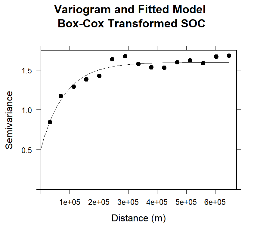

Ordinary kriging

ok.soc<-krige(SOC.bc~1, 
              train, 
              grid,
              model=m.f, 
              nmax=50
              )

## [using ordinary kriging]

# back transformation
k1<-1/0.2523339                                   
grid.xy$OK <-((ok.soc$var1.pred *0.2523339+1)^k1)

Conditional Gaussian Simulation

The krige() method can also do conditional simulations. It requires one optional argument: nsim, the number of conditional simulations

set.seed(130)
nsim=100
sim.soc<-krige(SOC.bc~1, 
              train, 
              grid,
              model=m.f, 
              nmax=50, 
              nsim = nsim)

## drawing 100 GLS realisations of beta...
## [using conditional Gaussian simulation]

Semiveriograms of All Realizations

Simulation is supposed to respect the spatial structure- same structure as the variogram model. Now will produce varigrams of 100 realization and plot them varigram of box-cox transform SOC.

plot(v$gamma ~ v$dist, xlim = c(0, max(v$dist) * 1.05),
ylim=c(0,2),
pch = 19, col = "black",cex=.5,
cex.axis = 0.8, cex.lab=1, xlab = list("Distance (m)",cex=1), ylab =list("Semivariance",cex=1),
main=list("Semi-variogram of 100 Realizations",cex=1))
for(i in 1:100) {
   sg.v=paste("sim",i,sep="")
   fg.v = as.formula(paste(sg.v, "~1"))
   vg.v = variogram(fg.v, sim.soc)
   lines(variogramLine(fit.variogram(vg.v, m.f),
   maxdist = max(v$dist)),lty=3, col = "grey")
}
points(v$gamma ~ v$dist,pch = 19, col = "red",cex=.3)
lines(variogramLine(fit.variogram(v,  m.f), 
maxdist = max(v$dist)), col = "red",  lwd=1.0)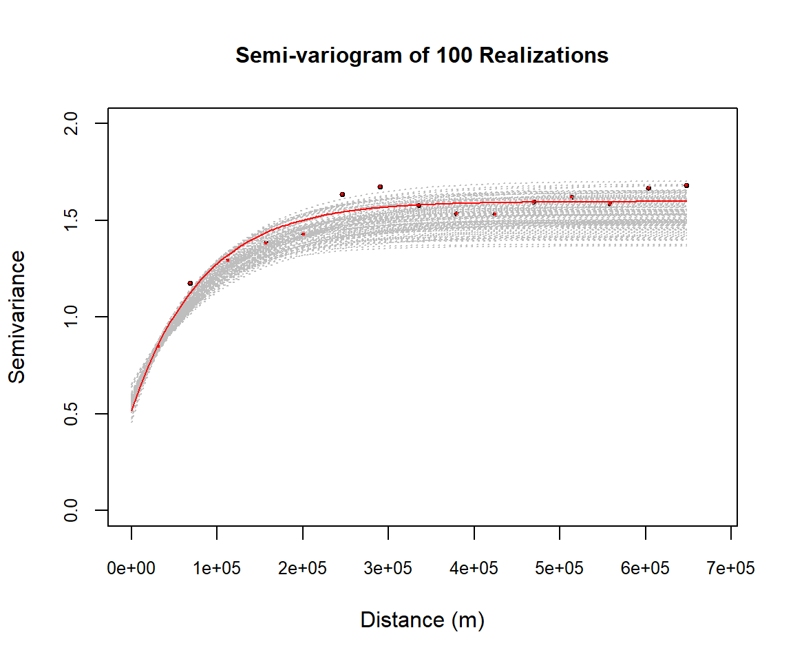

Back transformation

for(i in 1:length(sim.soc@data)){sim.soc@data[[i]] <- (((sim.soc[[i]]*0.2523339+1)^k1))}
sim.data<-as.data.frame(sim.soc)

Visualization of Spatial Uncetinity

The set of realizations provides a measure of uncertainty about the spatial distribution of arsenic concentration. Differences among the realizations describe the uncertainty. Such uncertainty can be visualized through an animated display of all realizations Which allows to distinguish areas that remain stable over all realizations (low uncertainty) from those where large fluctuations occur between realizations (high uncertainty).

Data preparation

soc=sim.data[,3:102]
soc.stack=stack(soc)
# round(quantile(soc.stack$values, probs=seq(0,1, by=.1)),1)
at.soc=classIntervals(soc.stack$values, n = 10, style = "quantile")$brks
rgb.palette <- colorRampPalette(c("red" ,"yellow","green","blue"),space = "rgb")
bound <- list("sp.lines", as(state, "SpatialLines"), col="grey40", lwd=.8,lty=1)
coordinates(sim.data) <- ~x+y
gridded(sim.data) <- TRUE

To create an animation map in R, you have to install animation packages in R. This package depends on ImageMagick software.

library(animation)

## Warning: package 'animation' was built under R version 3.6.2

After installation, you have define PATH of this software.

Sys.setenv(PATH = paste("C:\\Program Files\\ImageMagick-7.0.6-0-Q16", Sys.getenv("PATH"), sep = ";"))
ani.options(convert="C:\\Program Files\\ImageMagick-7.0.6-0-Q16\\covert.exe")
magickPath<-shortPathName("C:\\Program Files\\ImageMagick-7.0.6-0-Q16-x64\\magick.exe")
ani.options(convert=magickPath)

Animation Map

saveGIF(
for (i in 1:100){
print(spplot(sim.data[,i], main = list(label=paste("Realization",i),cex=1.5),
sp.layout=list(bound),
   par.settings=list(axis.line=list(col="grey25",lwd=0.5)),at=at.soc,
   colorkey=list(space="right",width=1.4,at=1:11,labels=list(cex=1.2,at=1:11,
   labels=c("",   "< 1.2",   "",   " 2.9", "",  " 4.7",  "",  " 7.2", "",  "> 12.5",  ""))),
   col.regions=rgb.palette(20)))}, 
height = 600, width = 600, interval = .5, outdir = getwd())

Measures of Local Uncertinity

Now, we will measure local uncertainty by comparing, E-tpye (mean), conditional qauntiles maps of expected probability of 10%, 50% (median) and 90%.

# E-type estimate
df<-as.data.frame(sim.data)
df<-df[,1:100]
grid.xy$mean<-as.data.frame(rowMeans(df[sapply(df, is.numeric)]))
names(grid.xy)[5]<-"Etype"
## Conditional Quantiles
grid.xy$q10<-apply(as.data.frame(sim.data)[3:102],1,stats::quantile,probs = 0.1,na.rm=TRUE) 
grid.xy$Median<-apply(as.data.frame(sim.data)[3:102],1,stats::quantile,probs = 0.5,na.rm=TRUE)
grid.xy$q90<-apply(as.data.frame(sim.data)[3:102],1,stats::quantile,probs = 0.9,na.rm=TRUE)

coordinates(grid.xy) <- ~x+y
gridded(grid.xy) <- TRUE

col <- colorRampPalette(c("red" ,"yellow","green","blue","sky blue"),space = "rgb")
spplot(grid.xy, c(4:5), sp.layout=list(bound), col.regions=col(20),
       names.attr = c("Ordinary Kriging", "E-type Estimates"))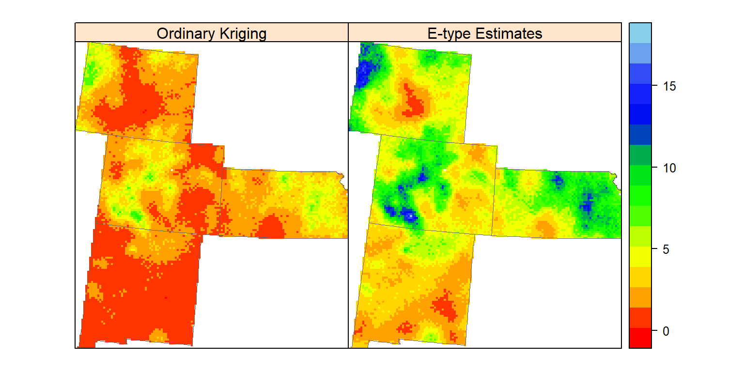

Ordinary predicted and E-type estimates of 100 realizations are not identical, although both are optimal of least-squares criterion.

Conditional Quantile Maps

spplot(grid.xy, c("q10","Median","q90"), sp.layout=list(bound), col.regions=col(20),
       names.attr = c("0.1-quantile", "Median","0.9 Quantile"))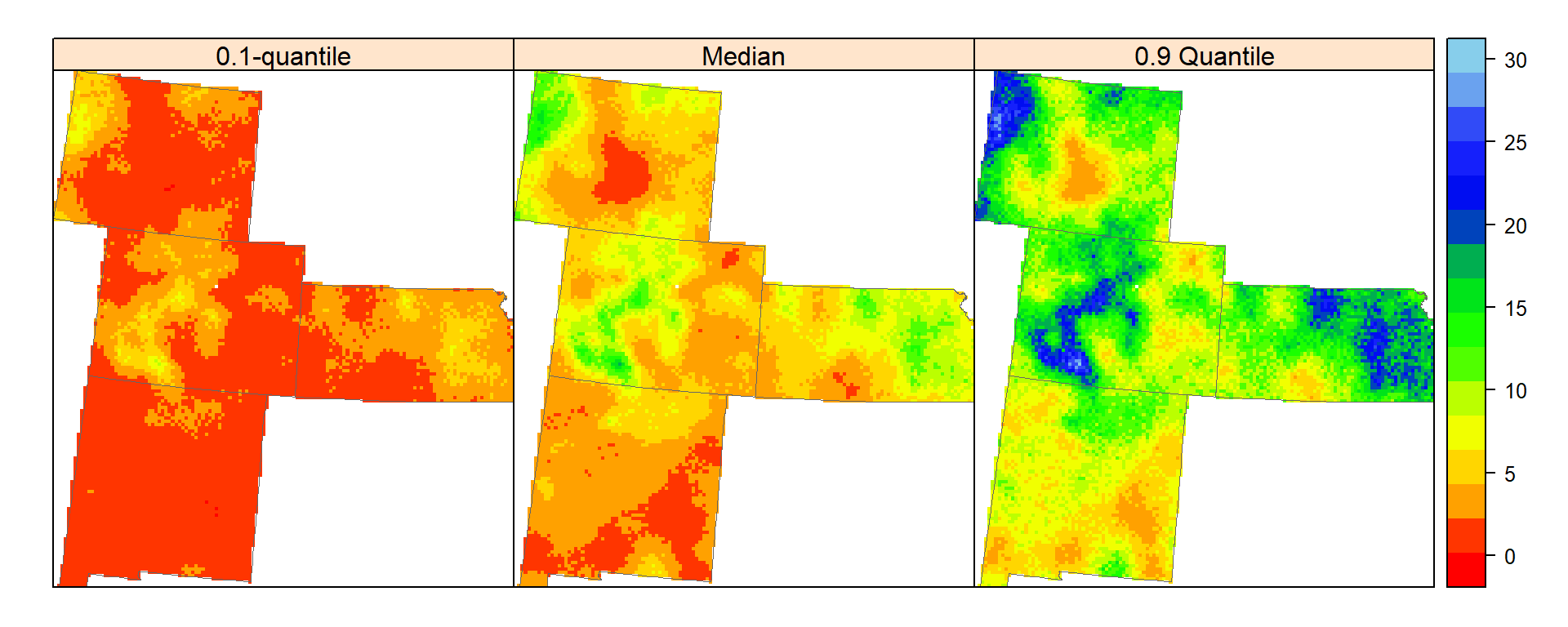

High Soil carbon (yellow part) of 0.1-quantile map indicate areas where unknown SOC concentration certainly large, whereas low value parts of (dark yellow) of the 0.9-qauntile map where concentration of SOC certainly small.

rm(list = ls())