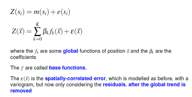
Universal Kriging
Universal Kriging (UK) is a variant of the Ordinary Kriging under non-stationary condition where mean differ in a deterministic way in different locations (trend or drift), while only the variance is constant.The trend can fitted range from local (immediate neighborhood) to global (whole area) This second-order stationarity (“weak stationarity”) is often a pertinent assumption with environmental exposures. In UK, usually first trend is calculated as a function of the coordinates and then the variation in what is left over (the residuals) as a random field is added to trend for making final prediction.
UK model the value of a variable at location as the sum of a regional non-stationary trend and a local spatially-correlated random component, the residuals from the regional trend.
Load package
library(plyr)
library(dplyr)
library(gstat)
library(raster)
library(ggplot2)
library(car)
library(classInt)
library(RStoolbox)
library(spatstat)
library(dismo)
library(fields)
library(gridExtra)
Load Data
The soil organic carbon data (train and test data set) could be found here.
# Define data folder
dataFolder<-"D:\\Dropbox\\Spatial Data Analysis and Processing in R\\DATA_08\\DATA_08\\"
train<-read.csv(paste0(dataFolder,"train_data.csv"), header= TRUE)
test<-read.csv(paste0(dataFolder,"test_data.csv"), header= TRUE)
state<-shapefile(paste0(dataFolder,"GP_STATE.shp"))
grid<-read.csv(paste0(dataFolder, "GP_prediction_grid_data.csv"), header= TRUE) Data Transformation
Power Transform uses the maximum likelihood-like approach of Box and Cox (1964) to select a transformation of a univariate or multivariate response for normality. First we have to calculate appropriate transformation parameters using powerTransform() function of car package and then use this parameter to transform the data using bcPower() function.
powerTransform(train$SOC)## Estimated transformation parameter
## train$SOC
## 0.2523339train$SOC.bc<-bcPower(train$SOC, 0.2523339)First. we have to define x & y variables to coordinates
coordinates(train) = ~x+y
coordinates(grid) = ~x+y
First, we will compute and visualize a first-order trend surface using krige() function.
trend<-krige(SOC.bc~x+y, train, grid, model=NULL)## [ordinary or weighted least squares prediction]trend.r<-rasterFromXYZ(as.data.frame(trend)[, c("x", "y", "var1.pred")])
ggR(trend.r, geom_raster = TRUE) +
scale_fill_gradientn("", colours = c("orange", "yellow", "green", "sky blue","blue"))+
theme_bw()+
theme(axis.title.x=element_blank(),
axis.text.x=element_blank(),
axis.ticks.x=element_blank(),
axis.title.y=element_blank(),
axis.text.y=element_blank(),
axis.ticks.y=element_blank())+
ggtitle("Global Trend of BoxCox-SOC")+
theme(plot.title = element_text(hjust = 0.5))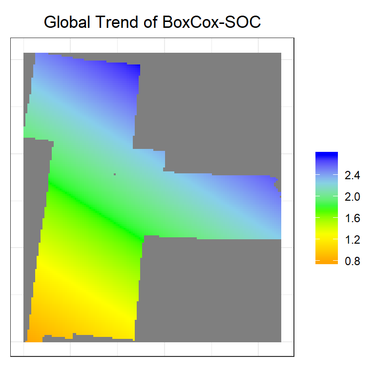
Variogram Modeling
In UK, the semivariances are based on the residuals, not the original data, because the random part of the spatial structure applies only to these residuals. The model parameters for the residuals will usually be very different from the original variogram model (often: lower sill, shorter range), since the global trend has taken out some of the variation and the long-range structure. In gstat, we can compute residual varoigram directly, if we provide an appropriate model formula; you do not have to compute the residuals manually.
We use the variogram method and specify the spatial dependence with the formula SOC.bc ~ x+y (as opposed to SOC.bc ~ 1 in the ordinary variogram). This has the same meaning as in the lm (linear regression) model specification: the SOC concentration is to be predicted using Ist order trend; then the residuals are to be modeled spatially.
# Variogram
v<-variogram(SOC.bc~ x+y, data = train, cloud=F)
# Intial parameter set by eye esitmation
m<-vgm(1.5,"Exp",40000,0.5)
# least square fit
m.f<-fit.variogram(v, m)
m.f
## model psill range
## 1 Nug 0.5186164 0.00
## 2 Exp 1.0744976 81954.85Plot Residuals varigram and Fitted model
#### Plot varigram and fitted model:
plot(v, pl=F,
     model=m.f,
     col="black",
     cex=0.9,
     lwd=0.5,
     lty=1,
     pch=19,
     main="Variogram of Residuals",
     xlab="Distance (m)",
     ylab="Semivariance")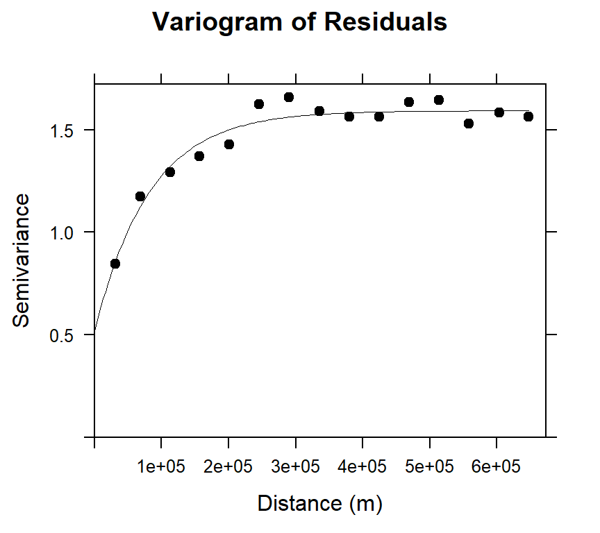
Kriging Prediction
krige() function in gstat package use for simple, ordinary or universal kriging (sometimes called external drift kriging), kriging in a local neighborhood, point kriging or kriging of block mean values (rectangular or irregular blocks), and conditional (Gaussian or indicator) simulation equivalents for all kriging varieties, and function for inverse distance weighted interpolation. For multivariate prediction.
UK<-krige(SOC.bc~x+y,
              loc= train,        # Data frame
              newdata=grid,      # Prediction grid
              model = m.f)       # fitted varigram model
## [using universal kriging]summary(UK)## Object of class SpatialPointsDataFrame
## Coordinates:
## min max
## x -1245285 114715
## y 1003795 2533795
## Is projected: NA
## proj4string : [NA]
## Number of points: 10674
## Data attributes:
## var1.pred var1.var
## Min. :-0.1549 Min. :0.7235
## 1st Qu.: 1.2799 1st Qu.:0.9298
## Median : 1.8873 Median :1.0023
## Mean : 1.8862 Mean :1.0244
## 3rd Qu.: 2.5169 3rd Qu.:1.1020
## Max. : 4.1413 Max. :1.4817Back transformation
We will back transformation using transformation parameters that have used Box-cos transformation
k1<-1/0.2523339
UK$UK.pred <-((UK$var1.pred *0.2523339+1)^k1)
UK$UK.var <-((UK$var1.var *0.2523339+1)^k1)
summary(UK)
## Object of class SpatialPointsDataFrame
## Coordinates:
## min max
## x -1245285 114715
## y 1003795 2533795
## Is projected: NA
## proj4string : [NA]
## Number of points: 10674
## Data attributes:
## var1.pred var1.var UK.pred UK.var
## Min. :-0.1549 Min. :0.7235 Min. : 0.8539 Min. :1.944
## 1st Qu.: 1.2799 1st Qu.:0.9298 1st Qu.: 3.0319 1st Qu.:2.305
## Median : 1.8873 Median :1.0023 Median : 4.6814 Median :2.444
## Mean : 1.8862 Mean :1.0244 Mean : 5.2142 Mean :2.497
## 3rd Qu.: 2.5169 3rd Qu.:1.1020 3rd Qu.: 7.0191 3rd Qu.:2.644
## Max. : 4.1413 Max. :1.4817 Max. :17.0323 Max. :3.521Convert to raster
UK.pred<-rasterFromXYZ(as.data.frame(UK)[, c("x", "y", "UK.pred")])
UK.var<-rasterFromXYZ(as.data.frame(UK)[, c("x", "y", "UK.var")])
Plot predicted SOC and OK Error
p1<-ggR(UK.pred, geom_raster = TRUE) +
scale_fill_gradientn("", colours = c("orange", "yellow", "green",  "sky blue","blue"))+
  theme_bw()+
    theme(axis.title.x=element_blank(),
        axis.text.x=element_blank(),
        axis.ticks.x=element_blank(),
        axis.title.y=element_blank(),
        axis.text.y=element_blank(),
        axis.ticks.y=element_blank())+
   ggtitle("UK Predicted SOC")+
   theme(plot.title = element_text(hjust = 0.5))

p2<-ggR(UK.var, geom_raster = TRUE) +
scale_fill_gradientn("", colours = c("blue",  "green","yellow", "orange"))+
  theme_bw()+
    theme(axis.title.x=element_blank(),
        axis.text.x=element_blank(),
        axis.ticks.x=element_blank(),
        axis.title.y=element_blank(),
        axis.text.y=element_blank(),
        axis.ticks.y=element_blank())+
   ggtitle("UK Predition Variance")+
   theme(plot.title = element_text(hjust = 0.5))

grid.arrange(p1,p2, ncol = 2) # Multiplot 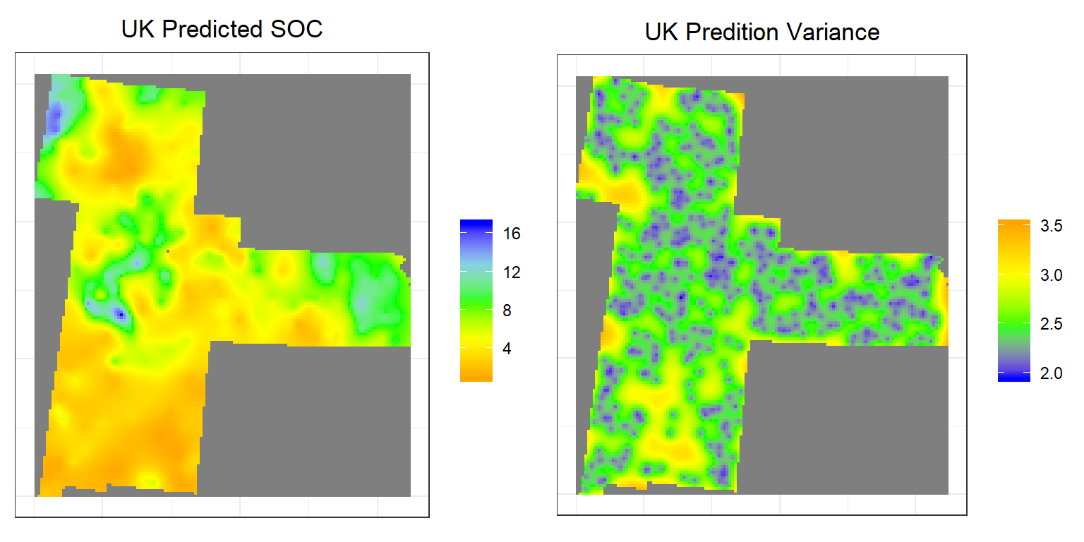
Above plots show the interpolated map of soil SOC with associated error at each prediction grid. OK predicted map shows global pattern and hot spot locations of SOC concentration. The kriging variance is higher in unsampled locations, since variance depends on geometry of the sampling locations with lower variance near sampling locations. This kriging variance also depends on co variance model but independent of data values.
rm(list = ls())