Support Vector Machines (SVMs)- Supervised Image Classification
Support Vector Machines (SVMs) are supervised learning algorithms used mostly for classification problems. SVM models apply non-linear functions to select the best relationship between the response variable and predictors by introducing kernels functions that map the independent variables to higher dimensional feature spaces . This approach typically leads to a better generalization of the chosen model on out-of-sample data . The principle behind an SVM classifier algorithm is to separate data into different classes using a hyperplane. The goal in choosing a hyperplane is to maximize the distance from the hyperplane to the nearest data point of either class . These nearest data points are known as Support Vectors.
Load R packages
library(caret)        # machine laerning
library(kernlab)      # support vector machine
library(rgdal)        # spatial data processing
library(raster)       # raster processing
library(plyr)         # data manipulation
library(dplyr)        # data manipulation
library(RStoolbox)    # ploting spatial data
library(RColorBrewer) # color
library(ggplot2)      # ploting
library(sp)           # spatial data
library(doParallel)   # Parallel processing
The data could be available for download from here.
# Define data folder
dataFolder<-"D://Dropbox//Spatial Data Analysis and Processing in R//DATA_09//DATA_09//"
Load data
train.df<-read.csv(paste0(dataFolder,".\\Sentinel_2\\train_data.csv"), header = T)
test.df<-read.csv(paste0(dataFolder,".\\Sentinel_2\\test_data.csv"), header = T)
Start foreach to parallelize for model fitting
mc <- makeCluster(detectCores())
registerDoParallel(mc)
Tunning prameters
myControl <- trainControl(method="repeatedcv",
                          number=3,
                          repeats=2,
                          returnResamp='all',
                          allowParallel=TRUE)
Train SVM model
We will use the train() function from the caret package with “method” parameter “svmRadial” (Radial Based Kernel based classification) wrapped from the Kernlab package.
set.seed(849)
fit.svm <- train(as.factor(Landuse)~B2+B3+B4+B4+B6+B7+B8+B8A+B11+B12,
                data=train.df,
                method = "svmRadial",
                metric= "Accuracy",
                preProc = c("center", "scale"),
                trControl = myControl
                )
fit.svm
## Support Vector Machines with Radial Basis Function Kernel
##
## 16764 samples
## 9 predictor
## 5 classes: 'Building', 'Grass', 'Parking/road/pavement', 'Tree/bushes', 'Water'
##
## Pre-processing: centered (9), scaled (9)
## Resampling: Cross-Validated (3 fold, repeated 2 times)
## Summary of sample sizes: 11175, 11176, 11177, 11175, 11177, 11176, ...
## Resampling results across tuning parameters:
##
## C Accuracy Kappa
## 0.25 0.9564543 0.9422039
## 0.50 0.9645668 0.9529613
## 1.00 0.9754235 0.9673634
##
## Tuning parameter 'sigma' was held constant at a value of 1.446147
## Accuracy was used to select the optimal model using the largest value.
## The final values used for the model were sigma = 1.446147 and C = 1.Stop cluster
stopCluster(mc)Confusion Matrix - train data
p1<-predict(fit.svm, train.df, type = "raw")
confusionMatrix(p1, train.df$Landuse)
## Confusion Matrix and Statistics
##
## Reference
## Prediction Building Grass Parking/road/pavement Tree/bushes
## Building 2984 0 50 0
## Grass 0 3442 0 21
## Parking/road/pavement 76 0 3812 63
## Tree/bushes 41 40 12 5584
## Water 0 0 0 0
## Reference
## Prediction Water
## Building 0
## Grass 0
## Parking/road/pavement 0
## Tree/bushes 13
## Water 626
##
## Overall Statistics
##
## Accuracy : 0.9812
## 95% CI : (0.979, 0.9832)
## No Information Rate : 0.3381
## P-Value [Acc > NIR] : < 2.2e-16
##
## Kappa : 0.975
##
## Mcnemar's Test P-Value : NA
##
## Statistics by Class:
##
## Class: Building Class: Grass
## Sensitivity 0.9623 0.9885
## Specificity 0.9963 0.9984
## Pos Pred Value 0.9835 0.9939
## Neg Pred Value 0.9915 0.9970
## Prevalence 0.1850 0.2077
## Detection Rate 0.1780 0.2053
## Detection Prevalence 0.1810 0.2066
## Balanced Accuracy 0.9793 0.9935
## Class: Parking/road/pavement Class: Tree/bushes
## Sensitivity 0.9840 0.9852
## Specificity 0.9892 0.9904
## Pos Pred Value 0.9648 0.9814
## Neg Pred Value 0.9952 0.9924
## Prevalence 0.2311 0.3381
## Detection Rate 0.2274 0.3331
## Detection Prevalence 0.2357 0.3394
## Balanced Accuracy 0.9866 0.9878
## Class: Water
## Sensitivity 0.97966
## Specificity 1.00000
## Pos Pred Value 1.00000
## Neg Pred Value 0.99919
## Prevalence 0.03812
## Detection Rate 0.03734
## Detection Prevalence 0.03734
## Balanced Accuracy 0.98983Confusion Matrix - test data
p2<-predict(fit.svm, test.df, type = "raw")
confusionMatrix(p2, test.df$Landuse)
## Confusion Matrix and Statistics
##
## Reference
## Prediction Building Grass Parking/road/pavement Tree/bushes
## Building 1273 0 16 0
## Grass 0 1478 0 8
## Parking/road/pavement 43 0 1639 18
## Tree/bushes 12 13 5 2403
## Water 0 0 0 0
## Reference
## Prediction Water
## Building 0
## Grass 0
## Parking/road/pavement 0
## Tree/bushes 5
## Water 268
##
## Overall Statistics
##
## Accuracy : 0.9833
## 95% CI : (0.9801, 0.9861)
## No Information Rate : 0.3383
## P-Value [Acc > NIR] : < 2.2e-16
##
## Kappa : 0.9778
##
## Mcnemar's Test P-Value : NA
##
## Statistics by Class:
##
## Class: Building Class: Grass
## Sensitivity 0.9586 0.9913
## Specificity 0.9973 0.9986
## Pos Pred Value 0.9876 0.9946
## Neg Pred Value 0.9907 0.9977
## Prevalence 0.1849 0.2076
## Detection Rate 0.1773 0.2058
## Detection Prevalence 0.1795 0.2069
## Balanced Accuracy 0.9779 0.9949
## Class: Parking/road/pavement Class: Tree/bushes
## Sensitivity 0.9873 0.9893
## Specificity 0.9890 0.9926
## Pos Pred Value 0.9641 0.9856
## Neg Pred Value 0.9962 0.9945
## Prevalence 0.2312 0.3383
## Detection Rate 0.2282 0.3346
## Detection Prevalence 0.2367 0.3395
## Balanced Accuracy 0.9882 0.9910
## Class: Water
## Sensitivity 0.98168
## Specificity 1.00000
## Pos Pred Value 1.00000
## Neg Pred Value 0.99928
## Prevalence 0.03802
## Detection Rate 0.03732
## Detection Prevalence 0.03732
## Balanced Accuracy 0.99084Predition at grid location
# read grid CSV file
grid.df<-read.csv(paste0(dataFolder,".\\Sentinel_2\\prediction_grid_data.csv"), header = T)
# Preddict at grid location
p3<-as.data.frame(predict(fit.svm, grid.df, type = "raw"))
# Extract predicted landuse class
grid.df$Landuse<-p3$predict
# Import lnaduse ID file
ID<-read.csv(paste0(dataFolder,".\\Sentinel_2\\Landuse_ID.csv"), header=T)
# Join landuse ID
grid.new<-join(grid.df, ID, by="Landuse", type="inner")
# Omit missing values
grid.new.na<-na.omit(grid.new)
Convert to raster
x<-SpatialPointsDataFrame(as.data.frame(grid.new.na)[, c("x", "y")], data = grid.new.na)
r <- rasterFromXYZ(as.data.frame(x)[, c("x", "y", "Class_ID")])
Plot Landuse Map:
# Color Palette
myPalette <- colorRampPalette(c("light grey","burlywood4", "forestgreen","light green", "dodgerblue"))
# Plot Map
LU<-spplot(r,"Class_ID", main="Supervised Image Classification: svmRadial" ,
      colorkey = list(space="right",tick.number=1,height=1, width=1.5,
              labels = list(at = seq(1,4.8,length=5),cex=1.0,
              lab = c("Road/parking/pavement" ,"Building", "Tree/buses", "Grass", "Water"))),
              col.regions=myPalette,cut=4)
LU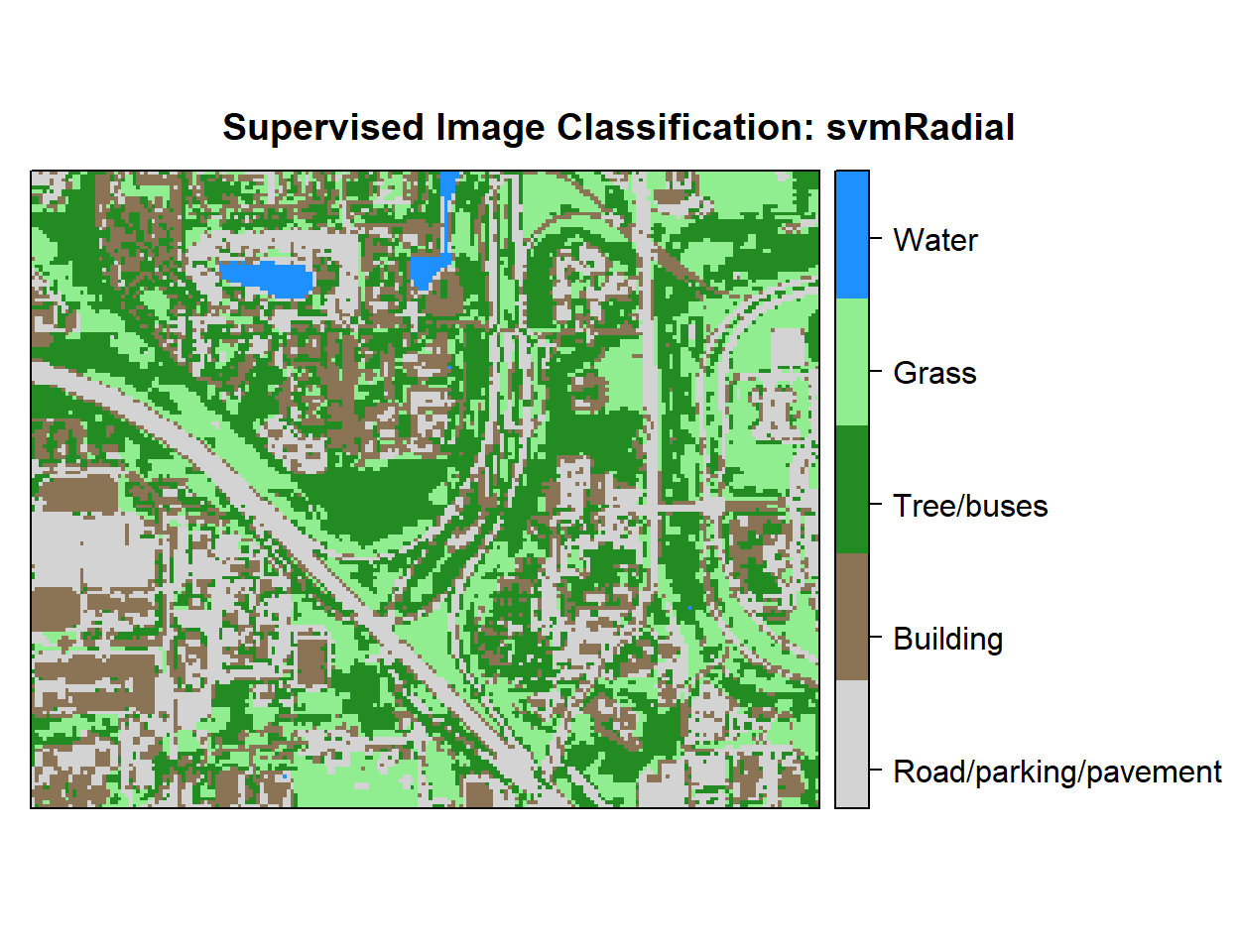
Write raster
# writeRaster(r, filename = paste0(dataFolder,".\\Sentinel_2\\SVM_Landuse.tiff"), "GTiff", overwrite=T)rm(list = ls())