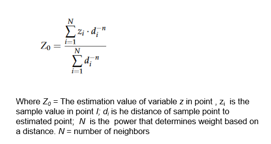
Deterministic Methods for Spatial Interpolation

Deterministic interpolation techniques, also known as exact interpolator, predict values from measured points, based on either the extent of similarity (inverse distance weighted) or the degree of smoothing (radial basis functions). This kind of interpolation techniques usually predict a value that is identical to the measured value at a sampled location without documenting potential error or error is assumed to be negligible.

Global techniques calculate predictions using the entire data set (Polynomial Trend Surface). Local techniques calculate predictions from the measured points within neighborhoods, which are smaller spatial areas within the larger study area.

In this exercise we will explore following deterministic methods to predict Soil Organic C:

Polynomial Trend Surface
Proximity Analysis-Thiessen Polygons
Nearest Neighbor Interpolation
Inverse Distance Weighted
Thin Plate Spline

Load package:

library(plyr)
library(dplyr)
library(gstat)
library(raster)
library(ggplot2)
library(car)
library(classInt)
library(RStoolbox)
library(spatstat)
library(dismo)
library(fields)

Load Data

The soil organic carbon data (train and test data set) could be found here.

# Define data folder
dataFolder<-"D:\\Dropbox\\Spatial Data Analysis and Processing in R\\DATA_08\\DATA_08\\"

train<-read.csv(paste0(dataFolder,"train_data.csv"), header= TRUE) 
state<-shapefile(paste0(dataFolder,"GP_STATE.shp"))
grid<-read.csv(paste0(dataFolder, "GP_prediction_grid_data.csv"), header= TRUE)

p.grid<-grid[,2:3]

Define coordinates

coordinates(train) = ~x+y
coordinates(grid) = ~x+y
gridded(grid) <- TRUE

Polynomial Trend Surface

Polynomial trend surfaces analysis is the most widely used global interpolation techniques where data is fitted with a least square equation (linear or quadratic equation), and then, interpolate surface is created based on this equation. The nature of the resulting surface is controlled by the order of the polynomial.

Linear fit

To fit a first order polynomial model:
SOC =intercept + aX+ bY (X = x coordinates, Y= y- coordinates)

We will use krige() function of gstat package without the geographic coordinates specified. It will perform ordinary or weighted least squares prediction

model.lm<-krige(SOC ~ x + y, train, grid)

## [ordinary or weighted least squares prediction]

summary(model.lm)

## Object of class SpatialPixelsDataFrame
## Coordinates:
##        min     max
## x -1250285  119715
## y   998795 2538795
## Is projected: NA 
## proj4string : [NA]
## Number of points: 10674
## Grid attributes:
##   cellcentre.offset cellsize cells.dim
## x          -1245285    10000       137
## y           1003795    10000       154
## Data attributes:
##    var1.pred        var1.var    
##  Min.   :2.726   Min.   :23.89  
##  1st Qu.:5.046   1st Qu.:23.94  
##  Median :6.480   Median :24.00  
##  Mean   :6.190   Mean   :24.03  
##  3rd Qu.:7.254   3rd Qu.:24.10  
##  Max.   :9.006   Max.   :24.39

Plot map

spplot(model.lm ,"var1.pred",
       main= "1st Order Trend Surface")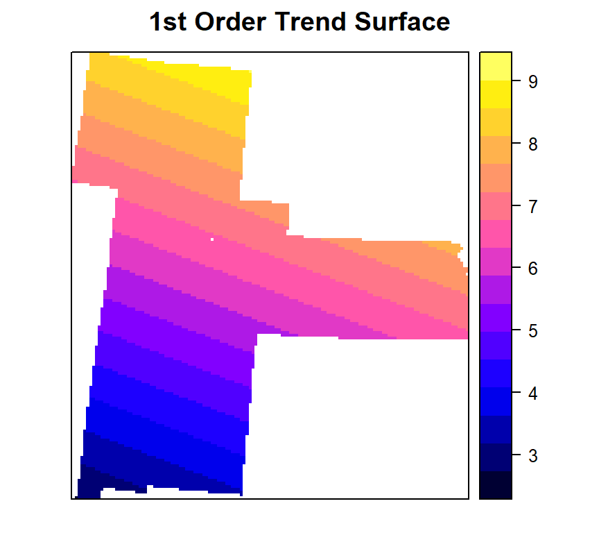

Quadratic Fit

To fit a second order polynomial model:

SOC = x + y + I(x*y) + I(x^2) + I(y^2)

model.quad<-krige(SOC ~ x + y + I(x*y) + I(x^2) + I(y^2), train, grid)

## [ordinary or weighted least squares prediction]

summary(model.quad)

## Object of class SpatialPixelsDataFrame
## Coordinates:
##        min     max
## x -1250285  119715
## y   998795 2538795
## Is projected: NA 
## proj4string : [NA]
## Number of points: 10674
## Grid attributes:
##   cellcentre.offset cellsize cells.dim
## x          -1245285    10000       137
## y           1003795    10000       154
## Data attributes:
##    var1.pred          var1.var    
##  Min.   : 0.6923   Min.   :21.84  
##  1st Qu.: 5.0919   1st Qu.:21.88  
##  Median : 6.0541   Median :21.96  
##  Mean   : 6.1666   Mean   :22.06  
##  3rd Qu.: 7.5374   3rd Qu.:22.17  
##  Max.   :11.5427   Max.   :23.52

Plot map

spplot(model.quad ,"var1.pred",
       main= "2nd Order Trend Surface")

Proximity Analysis-Thiessen Polygons

Thiessen polygons is the simplest interpolation method by which we can assign values at all unsampled locations considering the value of the closest sampled location. This way we can define boundaries of an area that is closest to each point relative to all other points. They are mathematically defined by the perpendicular bisectors of the lines between all points.

The Thiessen polygons can be created using ’s *dirichlet() function of spatstat or voronoi() function of dismo package in R

Here, we will apply voronoi function of dismo package

Before creating thiessen polygons, we have to create a SpatialPointsDataFrame

df<-as.data.frame(train)
##  define coordinates
xy <- df[,8:9]
SOC<-as.data.frame(df[,10])
names(SOC)[1]<-"SOC"
# Convert to spatial point
SPDF <- SpatialPointsDataFrame(coords = xy, data=SOC)

v <- voronoi(SPDF)
plot(v)

Plot looks not good, lets confined into GP state boundary.

# disslove inter-state boundary
bd <- aggregate(state)
# apply intersect fuction to clip
v.gp <- raster::intersect(v, bd)

## Warning in raster::intersect(v, bd): non identical CRS

Now we plot the maps

spplot(v.gp, 'SOC',
       main= "Thiessen polygons (Voronoi)",
       col.regions=rev(get_col_regions()))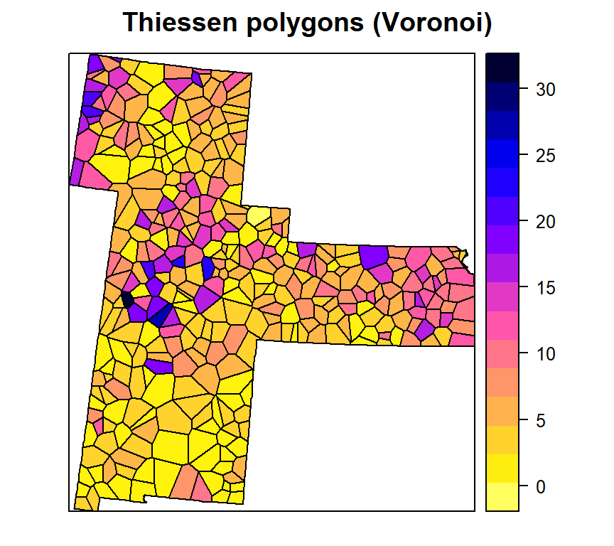

Now will convert this Voronoi polygon to raster (10 km x 10 km)

r <- raster(bd, res=10000)
vr <- rasterize(v.gp, r, 'SOC')

Plot map

ggR(vr, geom_raster = TRUE) +
  scale_fill_gradientn("SOC", colours = c("orange", "yellow", "green",  "blue","sky blue"))+
  theme_bw()+
    theme(axis.title.x=element_blank(),
        axis.text.x=element_blank(),
        axis.ticks.x=element_blank(),
        axis.title.y=element_blank(),
        axis.text.y=element_blank(),
        axis.ticks.y=element_blank())+
   ggtitle("Thiessen polygons (Voronoi) of SOC")+
   theme(plot.title = element_text(hjust = 0.5))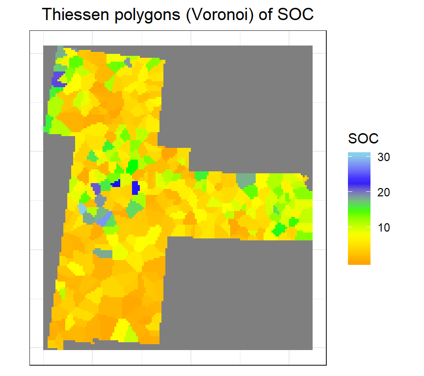

Nearest Neighbor Interpolation

Here we do nearest neighbor interpolation considering multiple (5) neighbors.

We will use the gstat package to interpolate SOC using Nearest Neighbor Interpolation. First we fit a model ( ~1 means) “intercept only” using krige() function. In the case of spatial data, that would be only ‘x’ and ‘y’ coordinates are used. We set the maximum number of points to 5, and the “inverse distance power” idp to zero, such that all five neighbors are equally weighted.

nn <- krige(SOC ~ 1, train, grid, nmax=5, set=list(idp = 0))

## [inverse distance weighted interpolation]

Convert to raster

nn.na<-na.omit(nn)
nn.pred<-rasterFromXYZ(as.data.frame(nn)[, c("x", "y", "var1.pred")])

Plot Nearest Neighbour predicted SOC

ggR(nn.pred, geom_raster = TRUE) +
  scale_fill_gradientn("SOC", colours = c("orange", "yellow", "green",  "sky blue","blue"))+
  theme_bw()+
    theme(axis.title.x=element_blank(),
        axis.text.x=element_blank(),
        axis.ticks.x=element_blank(),
        axis.title.y=element_blank(),
        axis.text.y=element_blank(),
        axis.ticks.y=element_blank())+
   ggtitle("Nearest Neighbour\n Predicted SOC")+
   theme(plot.title = element_text(hjust = 0.5))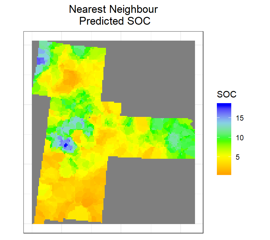

Inverse Distance Weighted Interpolation

Inverse distance weighted (IDW) is one of the most commonly used non-statistical method for spatial interpolation based on an assumption that things that are close to one another are more alike than those that are farther apart, and each measured point has a local influence that diminishes with distance. It gives greater weights to points closest to the prediction location, and the weights diminish as a function of distance. The factors that affect the accuracy of IWD are the value of the power parameter and size and the number of the neighbor.

We will use the gstat package to interpolate SOC using IDW. First we fit a model ( ~1 means) “intercept only” using krige() function. In the case of spatial data, that would be only ‘x’ and ‘y’ coordinates are used.

IDW<- krige(SOC ~ 1, train, grid)

## [inverse distance weighted interpolation]

summary(IDW)

## Object of class SpatialPixelsDataFrame
## Coordinates:
##        min     max
## x -1250285  119715
## y   998795 2538795
## Is projected: NA 
## proj4string : [NA]
## Number of points: 10674
## Grid attributes:
##   cellcentre.offset cellsize cells.dim
## x          -1245285    10000       137
## y           1003795    10000       154
## Data attributes:
##    var1.pred          var1.var    
##  Min.   : 0.4831   Min.   : NA    
##  1st Qu.: 4.2517   1st Qu.: NA    
##  Median : 5.7212   Median : NA    
##  Mean   : 6.1423   Mean   :NaN    
##  3rd Qu.: 7.6260   3rd Qu.: NA    
##  Max.   :29.0807   Max.   : NA    
##                    NA's   :10674

Convert to raster

idw.na<-na.omit(idw)
IDW.pred<-rasterFromXYZ(as.data.frame(IDW)[, c("x", "y", "var1.pred")])

Plot IDW predicted SOC

ggR(IDW.pred, geom_raster = TRUE) +
  scale_fill_gradientn("SOC", colours = c("orange", "yellow", "green",  "sky blue","blue"))+
  theme_bw()+
    theme(axis.title.x=element_blank(),
        axis.text.x=element_blank(),
        axis.ticks.x=element_blank(),
        axis.title.y=element_blank(),
        axis.text.y=element_blank(),
        axis.ticks.y=element_blank())+
   ggtitle("Inverse Distance Weighted (IDW)\n Predicted SOC")+
   theme(plot.title = element_text(hjust = 0.5))

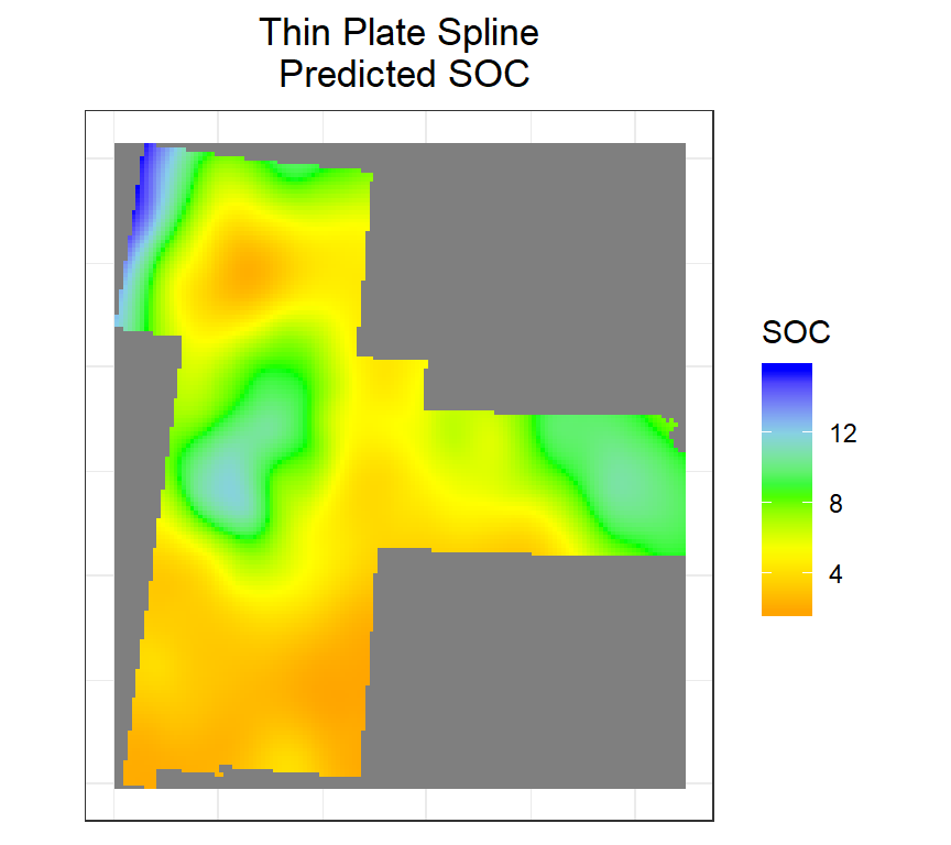
Thin Plate Spline

Thin Plate Splines are used to produce approximations to given data in more than one dimension. These are analogous to the cubic splines in one dimension. We can fits a thin plate spline surface to irregularly spaced spatial data.

We use Tps() function of field package to create thin plate spline surface

m <- Tps(coordinates(train), train$SOC)
tps <- interpolate(r, m)  
plot(tps)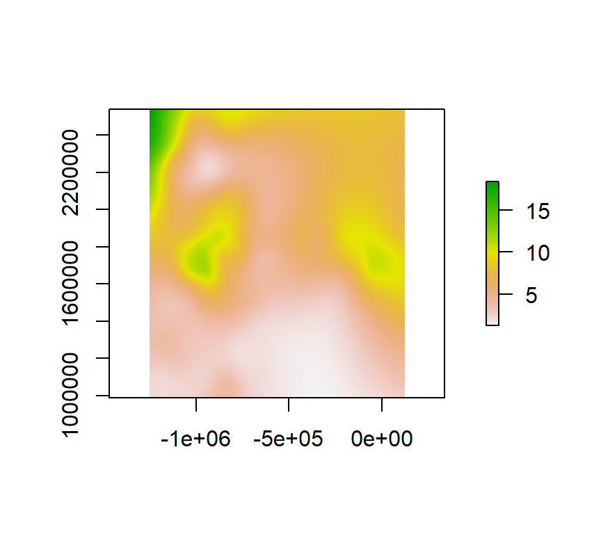

tps <- raster::mask(tps,bd) # mask out

ggR(tps, geom_raster = TRUE) +
  scale_fill_gradientn("SOC", colours = c("orange", "yellow", "green",  "sky blue","blue"))+
  theme_bw()+
    theme(axis.title.x=element_blank(),
        axis.text.x=element_blank(),
        axis.ticks.x=element_blank(),
        axis.title.y=element_blank(),
        axis.text.y=element_blank(),
        axis.ticks.y=element_blank())+
   ggtitle("Thin Plate Spline\n Predicted SOC")+
   theme(plot.title = element_text(hjust = 0.5))