Kriging
Kriging is a group of geostatistical techniques to interpolate the value of a random field (e.g., the soil variables as a function of the geographic location) at an un-sampled location from known observations of its value at nearby locations. The main statistical assumption behind kriging is one of stationarity which means that statistical properties (such as mean and variance) do not depend on the exact spatial locations, so the mean and variance of a variable at one location is equal to the mean and variance at another location. The basic idea of kriging is to predict the value at a given point by computing a weighted average of the known values of the function in the neighborhood of the point. Unlike other deterministic interpolation methods such as inverse distance weighted (IDW) and Spline, kriging is based on auto-correlation-that is, the statistical relationships among the measured points to interpolate the values in the spatial field. Kriging is capable to produce prediction surface with uncertainty. Although stationarity (constant mean and variance) and isotropy (uniformity in all directions) are the two main assumptions for kriging to provide best linear unbiased prediction, however, there is flexibility of these assumptions for various forms and methods of kriging.
Steps of kriging:
computation of average sample to sample variability of samples falling within the radius of search;
selection of nearest samples lying within the radius of search;
establishment of kriging matrices involving setting up of a semivariance matrix that contain expected sample variabilities for each of the neighborhood sample values, and setting up of a matrix that contain the average variability between each of the nearest neighborhood sample values and the block;
establishment of kriging coefficient matrix; and
multiplication of kriging coefficients by their respective sample values to provide kriged estimates (KE). The kriging variance (KV) is calculated from the sum of the products of the weight coefficients and their respective sample block variances. An extra constant, the lag-range multiplier is added to minimize the variance.
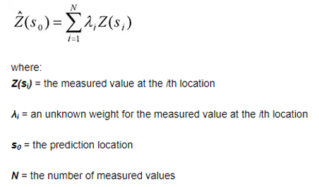
The weights are determined from the variogram based on the spatial structure of the data. The general formula for both interpolators is formed as a weighted sum of the data:
Types of Kriging
The six most common sub-types of kriging, including:
Ordinary kriging (OK)
Ordinary kriging (OK) is the most widely used kriging method. It is a linear unbiased estimators since error mean is equal to zero. In OK, local mean is filtered from the linear estimator by forcing the kriging weights to sum to 1. The OK is usually preferred to simple kriging because it requires neither knowledge nor stationarity of mean over the entire area
Universal Kriging (UK)
Universal Kriging (UK) is a variant of the Ordinary Kriging under non-stationary condition where mean differ in a deterministic way in different locations (local trend or drift), while only the variance is constant. This second-order stationarity (“weak stationarity”) is often a pertinent assumption with environmental exposures. In UK, usually first trend is calculated as a function of the coordinates and then the variation in what is left over (the residuals) as a random field is added to trend for making final prediction.
Co-Kriging (CK)
Co-kriging (CK) is an extension of ordinary kriging in which additional observed variables (know as co-variate which are often correlated with the variable of interest) are used to enhance the precision of the interpolation of the variable of interest. Unlike regression and universal kriging, Co-Kriging does not require that the secondary information is available at all prediction locations. The co-variable may be measured at the same points as the target (co-located samples), at other points, or both. The most common application of co-kriging is when the co-variable is cheaper to measure than the target variable.
Regression kriging
Regression kriging (RK) mathematically equivalent to the universal kriging or kriging with external drift, where auxiliary predictors are used directly to solve the kriging weights. Regression kriging combines a regression model with simple kriging of the regression residuals. The experimental variogram of residuals is first computed and modeled, and then simple kriging (SK) is applied to the residuals to give the spatial prediction of the residuals.
Indicator kriging
Indicator kriging (IK) is a non-parametric geostatistical method where environmental variables are discretized a range of variation by a set of thresholds (e.g. deciles of sample histogram, detection limit, regulatory threshold) and transformed each observation into a vector of indicators of non-exceedance of each threshold. Then, kriging is applied to the set of indicators and estimated values are assembled to form a conditional cumulative distribution function (ccdf). The mean or median of the probability distribution can be used as an estimate of the pollutant concentration. Indicator kriging provides a flexible interpolation approach that is well suited for data sets where: 1) many observations are below the detection limit, 2) the histogram is strongly skewed, or 3) specific classes of attribute values are better connected in space than others (e.g. low pollutant concentrations) (Goovaerts, 2009).
The OK, UK or RK interpolation methods can be applied in one of two forms Punctual/point or Block. Punctual Kriging (the default) estimates the value at a given point and is most commonly used. Block Kriging uses the estimate of the average expected value in a given location (such as a “block”) around a point. Block Kriging provides better variance estimation and has the effect of smoothing interpolated results.