Random Forest - Supervised Image Classification
Random forests are based on assembling multiple iterations of decision trees. They have become a major data analysis tool that performs well in comparison to single iteration classification and regression tree analysis [Heidema et al., 2006]. Each tree is made by bootstrapping a part of the original data set to estimate robust errors. The remaining data are used for testing; and this test data set, is called the Out-Of-Bag (OOB) sample. Within a given data set, the OOB sample values are predicted from the bootstrap samples. The predictions of the OOB values in all of the data sets are then combined. The Random Forest algorithm allows estimation of the importance of predictor variables by measuring the mean decrease in prediction accuracy before and after permuting OOB variables. The difference between the two are then averaged over all trees and normalized by the standard deviation of the differences. The Random Forest algorithm can outperform linear regression, and unlike linear regression, RF makes no assumptions about the probability density function of the predicted variable [Hengl et al., 2015; Kuhn and Johnson, 2013]. However, the major disadvantage of the Random Forest algorithm is that it is difficult to interpret the relationships between the predicted and predictor variables.
Load R packages
library(caret)        # machine laerning
library(randomForest) # Random Forest
library(rgdal)        # spatial data processing
library(raster)       # raster processing
library(plyr)         # data manipulation
library(dplyr)        # data manipulation
library(RStoolbox)    # ploting spatial data
library(RColorBrewer) # color
library(ggplot2)      # ploting
library(sp)           # spatial data
library(doParallel)   # Parallel processing
The data could be available for download from here.
# Define data folder
dataFolder<-"D://Dropbox//Spatial Data Analysis and Processing in R//DATA_09//DATA_09//"
Load data
train.df<-read.csv(paste0(dataFolder,".\\Sentinel_2\\train_data.csv"), header = T)
test.df<-read.csv(paste0(dataFolder,".\\Sentinel_2\\test_data.csv"), header = T)
Start foreach to parallelize for model fitting:
mc <- makeCluster(detectCores())
registerDoParallel(mc)
Tunning prameters
myControl <- trainControl(method="repeatedcv",
                          number=3,
                          repeats=2,
                          returnResamp='all',
                          allowParallel=TRUE)
Train Random Forest model
We will use train() function of caret package with “method” parameter “rf” wrapped from Random Forest package.
set.seed(849)
fit.rf <- train(as.factor(Landuse)~B2+B3+B4+B4+B6+B7+B8+B8A+B11+B12,
                data=train.df,
                method = "rf",
                metric= "Accuracy",
                preProc = c("center", "scale"),
                trControl = myControl
                )
fit.rf
## Random Forest
##
## 16764 samples
## 9 predictor
## 5 classes: 'Building', 'Grass', 'Parking/road/pavement', 'Tree/bushes', 'Water'
##
## Pre-processing: centered (9), scaled (9)
## Resampling: Cross-Validated (3 fold, repeated 2 times)
## Summary of sample sizes: 11175, 11176, 11177, 11175, 11177, 11176, ...
## Resampling results across tuning parameters:
##
## mtry Accuracy Kappa
## 2 0.9981807 0.9975852
## 5 0.9979123 0.9972289
## 9 0.9978825 0.9971893
##
## Accuracy was used to select the optimal model using the largest value.
## The final value used for the model was mtry = 2.Stop cluster
stopCluster(mc)Confusion Matrix - train data
p1<-predict(fit.rf, train.df, type = "raw")
confusionMatrix(p1, train.df$Landuse)
## Confusion Matrix and Statistics
##
## Reference
## Prediction Building Grass Parking/road/pavement Tree/bushes
## Building 3101 0 0 0
## Grass 0 3482 0 0
## Parking/road/pavement 0 0 3874 0
## Tree/bushes 0 0 0 5668
## Water 0 0 0 0
## Reference
## Prediction Water
## Building 0
## Grass 0
## Parking/road/pavement 0
## Tree/bushes 0
## Water 639
##
## Overall Statistics
##
## Accuracy : 1
## 95% CI : (0.9998, 1)
## No Information Rate : 0.3381
## P-Value [Acc > NIR] : < 2.2e-16
##
## Kappa : 1
##
## Mcnemar's Test P-Value : NA
##
## Statistics by Class:
##
## Class: Building Class: Grass
## Sensitivity 1.000 1.0000
## Specificity 1.000 1.0000
## Pos Pred Value 1.000 1.0000
## Neg Pred Value 1.000 1.0000
## Prevalence 0.185 0.2077
## Detection Rate 0.185 0.2077
## Detection Prevalence 0.185 0.2077
## Balanced Accuracy 1.000 1.0000
## Class: Parking/road/pavement Class: Tree/bushes
## Sensitivity 1.0000 1.0000
## Specificity 1.0000 1.0000
## Pos Pred Value 1.0000 1.0000
## Neg Pred Value 1.0000 1.0000
## Prevalence 0.2311 0.3381
## Detection Rate 0.2311 0.3381
## Detection Prevalence 0.2311 0.3381
## Balanced Accuracy 1.0000 1.0000
## Class: Water
## Sensitivity 1.00000
## Specificity 1.00000
## Pos Pred Value 1.00000
## Neg Pred Value 1.00000
## Prevalence 0.03812
## Detection Rate 0.03812
## Detection Prevalence 0.03812
## Balanced Accuracy 1.00000Confusion Matrix - test data
p2<-predict(fit.rf, test.df, type = "raw")
confusionMatrix(p2, test.df$Landuse)
## Confusion Matrix and Statistics
##
## Reference
## Prediction Building Grass Parking/road/pavement Tree/bushes
## Building 1328 0 0 0
## Grass 0 1491 0 0
## Parking/road/pavement 0 0 1660 0
## Tree/bushes 0 0 0 2429
## Water 0 0 0 0
## Reference
## Prediction Water
## Building 0
## Grass 0
## Parking/road/pavement 0
## Tree/bushes 0
## Water 273
##
## Overall Statistics
##
## Accuracy : 1
## 95% CI : (0.9995, 1)
## No Information Rate : 0.3383
## P-Value [Acc > NIR] : < 2.2e-16
##
## Kappa : 1
##
## Mcnemar's Test P-Value : NA
##
## Statistics by Class:
##
## Class: Building Class: Grass
## Sensitivity 1.0000 1.0000
## Specificity 1.0000 1.0000
## Pos Pred Value 1.0000 1.0000
## Neg Pred Value 1.0000 1.0000
## Prevalence 0.1849 0.2076
## Detection Rate 0.1849 0.2076
## Detection Prevalence 0.1849 0.2076
## Balanced Accuracy 1.0000 1.0000
## Class: Parking/road/pavement Class: Tree/bushes
## Sensitivity 1.0000 1.0000
## Specificity 1.0000 1.0000
## Pos Pred Value 1.0000 1.0000
## Neg Pred Value 1.0000 1.0000
## Prevalence 0.2312 0.3383
## Detection Rate 0.2312 0.3383
## Detection Prevalence 0.2312 0.3383
## Balanced Accuracy 1.0000 1.0000
## Class: Water
## Sensitivity 1.00000
## Specificity 1.00000
## Pos Pred Value 1.00000
## Neg Pred Value 1.00000
## Prevalence 0.03802
## Detection Rate 0.03802
## Detection Prevalence 0.03802
## Balanced Accuracy 1.00000Predition at grid location
# read grid CSV file
grid.df<-read.csv(paste0(dataFolder,".\\Sentinel_2\\prediction_grid_data.csv"), header = T)
# Preddict at grid location
p3<-as.data.frame(predict(fit.rf, grid.df, type = "raw"))
# Extract predicted landuse class
grid.df$Landuse<-p3$predict
# Import lnaduse ID file
ID<-read.csv(paste0(dataFolder,".\\Sentinel_2\\Landuse_ID.csv"), header=T)
# Join landuse ID
grid.new<-join(grid.df, ID, by="Landuse", type="inner")
# Omit missing values
grid.new.na<-na.omit(grid.new)
Convert to raster
x<-SpatialPointsDataFrame(as.data.frame(grid.new.na)[, c("x", "y")], data = grid.new.na)
r <- rasterFromXYZ(as.data.frame(x)[, c("x", "y", "Class_ID")])
Plot Landuse Map:
# Color Palette
myPalette <- colorRampPalette(c("light grey","burlywood4", "forestgreen","light green", "dodgerblue"))
# Plot Map
LU<-spplot(r,"Class_ID", main="Supervised Image Classification: Random Forest" ,
      colorkey = list(space="right",tick.number=1,height=1, width=1.5,
              labels = list(at = seq(1,4.8,length=5),cex=1.0,
              lab = c("Road/parking/pavement" ,"Building", "Tree/buses", "Grass", "Water"))),
              col.regions=myPalette,cut=4)
LU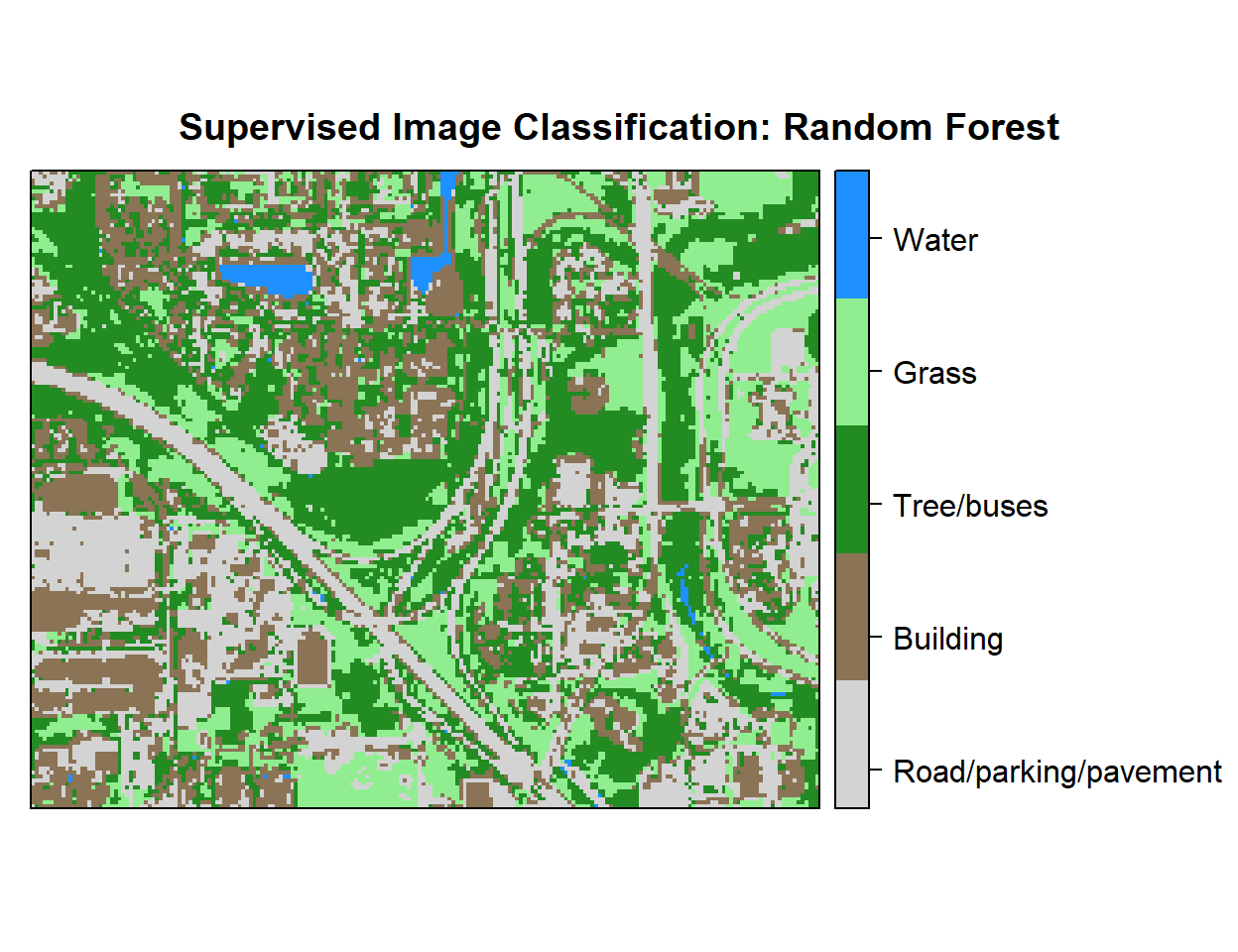
Write raster:
# writeRaster(r, filename = paste0(dataFolder,".\\Sentinel_2\\RF_Landuse.tiff"), "GTiff", overwrite=T)rm(list = ls())