Map Projection and Coordinate Reference Systems
The coordinate reference system (CRS) or spatial reference system (SRS) is a coordinate based system used to locate features on the earth.
Map projections is a systematic transformation a location on the surface of the earth or a portion of the earth (sphere or an ellipsoid) into on a plane (flat piece of paper or computer screen).

Map Projection (Source: (https://www.statcan.gc.ca/pub/92-195-x/2011001/other-autre/mapproj-projcarte/m-c-eng.htm)
We will cover following topics:
Geographic coordinate system (GCS)
Geographic coordinate systems use latitude and longitude to measure and locate feature on the globe. The GCS defines a position as a function of direction and distance from a center point of the globe, where the units of measurement are degrees. Any location on earth can be referenced by a point with longitude and latitude coordinates. For example, below figure shows a geographic coordinate system where a location is represented by the coordinate’s longitude 80 degree East and latitude 55 degree North.
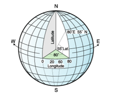
A Geographic coordinate system. (Source: http://www.ibm.com/support/knowledgecenter/SSEPGG_10.1.0/com.ibm.db2.luw.spatial.topics.doc/doc/csb3022a.html)
The equidistant lines that run east and west each have a constant latitude value called parallels. The equator is the largest circle and divides the earth in half. It is equal in distance from each of the poles, and the value of this latitude line is zero. Locations north of the equator has positive latitudes that range from 0 to +90 degrees, while locations south of the equator have negative latitudes that range from 0 to -90 degrees.
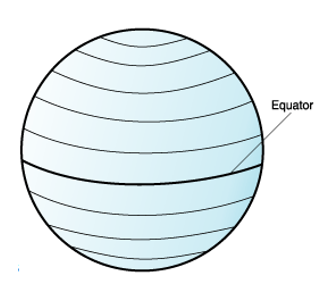
Latitude lines. (Source: http://www.ibm.com/support/knowledgecenter/SSEPGG_10.1.0/com.ibm.db2.luw.spatial.topics.doc/doc/csb3022a.html)
The lines that run through north and south each have a constant longitude value and form circles of the same size around the earth known as meridians. The prime meridian is the line of longitude that defines the origin (zero degrees) for longitude coordinates. One of the most commonly used prime meridian locations is the line that passes through Greenwich, England. Locations east of the prime meridian up to its antipodal meridian (the continuation of the prime meridian on the other side of the globe) have positive longitudes ranging from 0 to +180 degrees. Locations west of the prime meridian has negative longitudes ranging from 0 to -180 degrees.
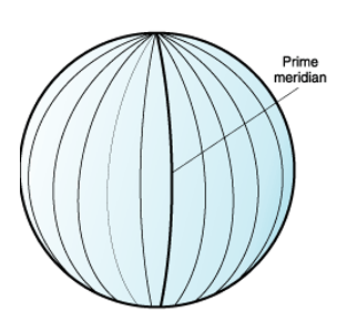
Longitude lines. (Source: http://www.ibm.com/support/knowledgecenter/SSEPGG_10.1.0/com.ibm.db2.luw.spatial.topics.doc/doc/csb3022a.html)
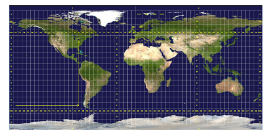
The latitude and longitude lines cover the globe to form a grid that know as a graticule. The point of origin of the graticule is (0,0), where the equator and the prime meridian intersect. The equator is the only place on the graticule where the linear distance corresponding to one degree latitude is approximately equal the distance corresponding to one degree longitude. Because the longitude lines converge at the poles, the distance between two meridians is different at every parallel.
The World Geodetic system 84
The most recent geographic coordinate system is the World Geodetic system 84 also known as WGS 1984 or EPSG:4326 (EPSG- European Petroleum Survey Group). It consists of a standard coordinate system, spheroidal reference (the datum or reference ellipsoid) and raw altitude.
The parameters of WGS84:
# GEOGCS["WGS 84",
#    DATUM["WGS_1984",
#      SPHEROID["WGS 84",6378137,298.257223563,
#            AUTHORITY["EPSG","7030"]],
#            AUTHORITY["EPSG","6326"]],
#      PRIMEM["Greenwich",0,
#      AUTHORITY["EPSG","8901"]],
#    UNIT["degree",0.01745329251994328,
#      AUTHORITY["EPSG","9122"]],
#    AUTHORITY["EPSG","4326"]]
Projected coordinate system
A projected coordinate system provide mechanisms to project maps of the earth’s spherical surface onto a two-dimensional Cartesian coordinate (x,y coordinates) plane. Projected coordinate systems are referred to as map projections. This approach is useful where accurate distance, angle, and area measurements are needed. The term ‘projection’ is often used interchangeably with projected coordinate systems.
Commonly use projected coordinate systems include:
Universal Transverse Mercator
The most widely used two-dimensional Cartesian coordinate system is the Universal Transverse Mercator (UTM) system which represents a horizontal position on the globe and can be used to identify positions without having to know their vertical location on the ‘y’ axis. The UTM system is not a single map projection. It represents the earth as sixty different zones, each composed of six-degree longitudinal bands, with a secant transverse Mercator projection in each. The UTM system divides the Earth between 80 S and 84 N latitude into 60 zones, each 6 of longitude in width. Zone 1 covers longitude 180 to 174 W; zone numbering increases eastward to zone 60, which covers longitude 174 to 180?.
UTM zones.(Source: https://en.wikipedia.org/wiki/Universal_Transverse_Mercator_coordinate_system)
The Universal Transverse Mercator grid that covers the conterminous 48 United States comprises 10 zones, from Zone 10 on the west coast through Zone 19 in New England USGS, 2001.The New York State falls in zones 17N (EPSG 26917) and zone 18N (EPSG: 26918) with North American Datum 1983 (NAD83).
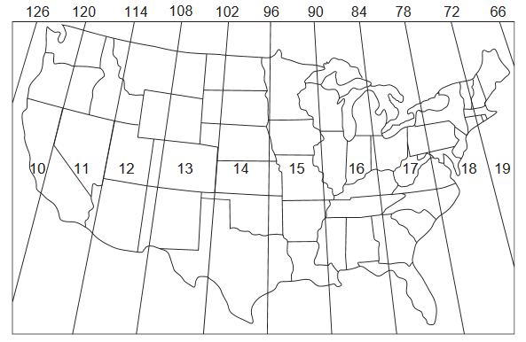
UTM zones of conterminous 48 United States. (Source: https://pubs.usgs.gov/fs/2001/0077/report.pdf)
The standard Parameters of UTM Zone 17N:
# PROJCS["NAD83 / UTM zone 17N",
#    GEOGCS["NAD83",
#        DATUM["North_American_Datum_1983",
#            SPHEROID["GRS 1980",6378137,298.257222101,
#                AUTHORITY["EPSG","7019"]],
#            AUTHORITY["EPSG","6269"]],
#        PRIMEM["Greenwich",0,
#            AUTHORITY["EPSG","8901"]],
#        UNIT["degree",0.01745329251994328,
#            AUTHORITY["EPSG","9122"]],
#        AUTHORITY["EPSG","4269"]],
#    UNIT["metre",1,
#        AUTHORITY["EPSG","9001"]],
#    PROJECTION["Transverse_Mercator"],
#    PARAMETER["latitude_of_origin",0],
#    PARAMETER["central_meridian",-81],
#    PARAMETER["scale_factor",0.9996],
#    PARAMETER["false_easting",500000],
#    PARAMETER["false_northing",0],
#    AUTHORITY["EPSG","26917"],
#    AXIS["Easting",EAST],
#    AXIS["Northing",NORTH]]
PROJ4 format
# +proj=utm +zone=17 +ellps=GRS80 +datum=NAD83 +units=m +no_defs ESRI .PROJ format
# WGS_1984_UTM_Zone_17N
# WKID: 32617 Authority: EPSG

# Projection: Transverse_Mercator
# False_Easting: 500000.0
# False_Northing: 0.0
# Central_Meridian: -81.0
# Scale_Factor: 0.9996
# Latitude_Of_Origin: 0.0
# Linear Unit: Meter (1.0)

# Geographic Coordinate System: GCS_WGS_1984
# Angular Unit: Degree (0.0174532925199433)
# Prime Meridian: Greenwich (0.0)
# Datum: D_WGS_1984
#  Spheroid: WGS_1984
#    Semimajor Axis: 6378137.0
#    Semiminor Axis: 6356752.314245179
#    Inverse Flattening: 298.257223563
The Standard Parameters of UTM Zone 18N:
# PROJCS["NAD83 / UTM zone 18N",
#    GEOGCS["NAD83",
#        DATUM["North_American_Datum_1983",
#            SPHEROID["GRS 1980",6378137,298.257222101,
#                AUTHORITY["EPSG","7019"]],
#            AUTHORITY["EPSG","6269"]],
#        PRIMEM["Greenwich",0,
#            AUTHORITY["EPSG","8901"]],
#        UNIT["degree",0.01745329251994328,
#            AUTHORITY["EPSG","9122"]],
#        AUTHORITY["EPSG","4269"]],
#    UNIT["metre",1,
#        AUTHORITY["EPSG","9001"]],
#    PROJECTION["Transverse_Mercator"],
#    PARAMETER["latitude_of_origin",0],
#    PARAMETER["central_meridian",-75],
#    PARAMETER["scale_factor",0.9996],
#    PARAMETER["false_easting",500000],
#    PARAMETER["false_northing",0],
#    AUTHORITY["EPSG","26918"],
#    AXIS["Easting",EAST],
#    AXIS["Northing",NORTH]]
PROJ4 format
# +proj=utm +zone=18 +ellps=GRS80 +datum=NAD83 +units=m +no_defs ESRI .PROJ format
# NAD_1983_2011_UTM_Zone_18N
# WKID: 6347 Authority: EPSG

# Projection: Transverse_Mercator
# False_Easting: 500000.0
# False_Northing: 0.0
# Central_Meridian: -75.0
# Scale_Factor: 0.9996
# Latitude_Of_Origin: 0.0
# Linear Unit: Meter (1.0)

# Geographic Coordinate System: GCS_WGS_1984
# Angular Unit: Degree (0.0174532925199433)
# Prime Meridian: Greenwich (0.0)
# Datum: D_WGS_1984
#  Spheroid: WGS_1984
#    Semimajor Axis: 6378137.0
#    Semiminor Axis: 6356752.314245179
#    Inverse Flattening: 298.257223563
Albers Equal Area Conic
Albers Equal Area Conic projection system uses two standard parallels to reduce the distortion of shape in the region between the standard parallels. This projection is best suited for area extending in an east-to-west orientation like the conterminous United States. Used for the conterminous United States, normally using 29-30 and 45-30 as the two standard parallels. For this projection, the maximum scale distortion for the 48 states of the conterminous United States is 1.25 percent.
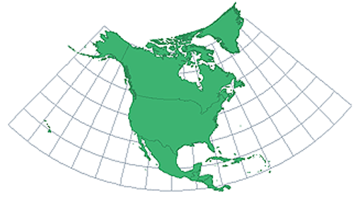
Albers Equal Area Conic. (Source: http://www.georeference.org/doc/albers_conical_equal_area.htm)
The Standard Parameters of Albers Equal Area Conic NAD1983 (ESRI:102003):
# PROJCS["USA_Contiguous_Albers_Equal_Area_Conic",
#    GEOGCS["GCS_North_American_1983",
#        DATUM["North_American_Datum_1983",
#            SPHEROID["GRS_1980",6378137,298.257222101]],
#        PRIMEM["Greenwich",0],
#        UNIT["Degree",0.017453292519943295]],
#    PROJECTION["Albers_Conic_Equal_Area"],
#    PARAMETER["False_Easting",0],
#    PARAMETER["False_Northing",0],
#    PARAMETER["longitude_of_center",-96],
#    PARAMETER["Standard_Parallel_1",29.5],
#    PARAMETER["Standard_Parallel_2",45.5],
#    PARAMETER["latitude_of_center",37.5],
#    UNIT["Meter",1],
#    AUTHORITY["EPSG","102003"]]
PROJ4 format
# +proj=aea +lat_1=29.5 +lat_2=45.5 +lat_0=37.5 +lon_0=-96 +x_0=0 +y_0=0 +datum=NAD83 +units=m +no_defs ESRI .PRJ format
# USA_Contiguous_Albers_Equal_Area_Conic
# WKID: 102003 Authority: Esri

# Projection: Albers
# False_Easting: 0.0
# False_Northing: 0.0
# Central_Meridian: -96.0
# Standard_Parallel_1: 29.5
# Standard_Parallel_2: 45.5
# Latitude_Of_Origin: 37.5
# Linear Unit: Meter (1.0)

# Geographic Coordinate System: GCS_North_American_1983
# Angular Unit: Degree (0.0174532925199433)
# Prime Meridian: Greenwich (0.0)
# Datum: D_North_American_1983
#  Spheroid: GRS_1980
#  Semimajor Axis: 6378137.0
#  Semiminor Axis: 6356752.314140356
#  Inverse Flattening: 298.257222101
Coordinate Reference System in R
In this exercise, we will learn how to check and define CRS and projection of vector and raster data in R. This is a very important step for working with geospatial data with different projection systems from different sources.
R Packages
Load R-packages
You need to load raster, and rgdal packages. Use library () functions to load them in R.
library(raster)
library (rgdal)
library(sf)
library(maptools)
Load Data
We will use following data set which could be found here.
- New York State county shape file (polygon: NY_County_GCS)
- 90 m SRTM DEM of Onondaga county, New York State (raster: Onondaga_DEM.tif)
Before reading the data from a local drive, you need to define a working directory from where you want to read or to write data. We will use setwd() function to create a working directory. Or we can define a path for data outside of our working directory from where we can read files. In this case, we will use paste0(path, “file name”)
#### Set working directory
# setwd("~//map_projection_coordinate_reference_systems")
# Define data folder
dataFolder<-"D://Dropbox//Spatial Data Analysis and Processing in R//DATA_03//DATA_03//"Vector data
We will use New York State County Shape file (NY_County_GCS.shp) to check, define projection. We will use shapefile() function of raster package to load Vector data in R.
poly.GCS<-readShapePoly(paste0(dataFolder, “NY_County_GCS.shp”))
county.GCS<-readShapePoly(paste0(dataFolder, "NY_County_GCS.shp"))
## Warning: readShapePoly is deprecated; use rgdal::readOGR or sf::st_read
plot(county.GCS,  main="NYS County")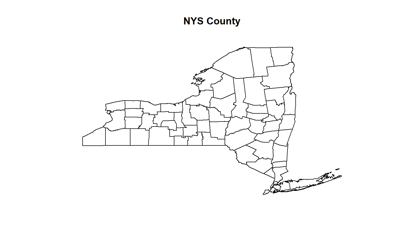
You notice that .prj file is not associated with this shape file. We can check further with proj4string() function.
proj4string(county.GCS)## [1] NAWe know that county shape file is in geographic coordinate system. We can check it coordinates system with summary() function.
summary(county.GCS)## Object of class SpatialPolygonsDataFrame
## Coordinates:
## min max
## x -79.76333 -71.85588
## y 40.49909 45.01100
## Is projected: NA
## proj4string : [NA]
## Data attributes:
## OBJECTID ID AREA PERIMETER
## 1 : 1 Min. :4770 Min. :0.0000 Min. :0.071
## 10 : 1 1st Qu.:5134 1st Qu.:0.0080 1st Qu.:0.518
## 11 : 1 Median :5263 Median :0.1510 Median :1.866
## 12 : 1 Mean :5279 Mean :0.1672 Mean :1.747
## 13 : 1 3rd Qu.:5455 3rd Qu.:0.2515 3rd Qu.:2.483
## 14 : 1 Max. :5756 Max. :0.8080 Max. :6.986
## (Other):77
## COUNTYP020 STATE COUNTY FIPS STATE_FIPS
## Min. :1876 NY:83 Suffolk County : 8 36103 : 8 36:83
## 1st Qu.:2240 Jefferson County : 7 36045 : 7
## Median :2369 Saint Lawrence County: 5 36089 : 5
## Mean :2385 Queens County : 3 36081 : 3
## 3rd Qu.:2561 Erie County : 2 36029 : 2
## Max. :2862 Nassau County : 2 36059 : 2
## (Other) :56 (Other):56
## SQUARE_MIL Shape_Leng Shape_Area
## Min. : 27.24 Min. : 6777 Min. :2.244e+06
## 1st Qu.: 496.44 1st Qu.: 51266 1st Qu.:7.206e+07
## Median : 839.97 Median :172376 Median :1.364e+09
## Mean : 907.23 Mean :164634 Mean :1.515e+09
## 3rd Qu.:1209.20 3rd Qu.:233235 3rd Qu.:2.314e+09
## Max. :2756.53 Max. :645199 Max. :7.142e+09
## You notice that county shape file read as SpatialPolygonsDataFrame in R, and it’s x-coordinates range from -79.76333 to -71.85588, and y-coordinates range from 40.49909 and 45.01100 and CRS has not been be defined yet (Is projected: NA and proj4string : [NA]) and .PRJ file is missing. So you need to define its current CRS (WGS 1984 or EPSG:4326) before you do any further analyses like re-projection etc. We use either of following function to define it’s CRS.
proj4string(county.GCS) = CRS("+proj=longlat +ellps=WGS84")
# or
proj4string(county.GCS) <- CRS("+init=epsg:4326")
## Warning in `proj4string<-`(`*tmp*`, value = new("CRS", projargs = "+init=epsg:4326 +proj=longlat +datum=WGS84 +no_defs +ellps=WGS84 +towgs84=0,0,0")): A new CRS was assigned to an object with an existing CRS:
## +proj=longlat +ellps=WGS84
## without reprojecting.
## For reprojection, use function spTransform
A new CRS, WGS 1984 has assigned to county shape file. You can check it again with summary() or str() functions.
summary (county.GCS)## Object of class SpatialPolygonsDataFrame
## Coordinates:
## min max
## x -79.76333 -71.85588
## y 40.49909 45.01100
## Is projected: FALSE
## proj4string :
## [+init=epsg:4326 +proj=longlat +datum=WGS84 +no_defs +ellps=WGS84
## +towgs84=0,0,0]
## Data attributes:
## OBJECTID ID AREA PERIMETER
## 1 : 1 Min. :4770 Min. :0.0000 Min. :0.071
## 10 : 1 1st Qu.:5134 1st Qu.:0.0080 1st Qu.:0.518
## 11 : 1 Median :5263 Median :0.1510 Median :1.866
## 12 : 1 Mean :5279 Mean :0.1672 Mean :1.747
## 13 : 1 3rd Qu.:5455 3rd Qu.:0.2515 3rd Qu.:2.483
## 14 : 1 Max. :5756 Max. :0.8080 Max. :6.986
## (Other):77
## COUNTYP020 STATE COUNTY FIPS STATE_FIPS
## Min. :1876 NY:83 Suffolk County : 8 36103 : 8 36:83
## 1st Qu.:2240 Jefferson County : 7 36045 : 7
## Median :2369 Saint Lawrence County: 5 36089 : 5
## Mean :2385 Queens County : 3 36081 : 3
## 3rd Qu.:2561 Erie County : 2 36029 : 2
## Max. :2862 Nassau County : 2 36059 : 2
## (Other) :56 (Other):56
## SQUARE_MIL Shape_Leng Shape_Area
## Min. : 27.24 Min. : 6777 Min. :2.244e+06
## 1st Qu.: 496.44 1st Qu.: 51266 1st Qu.:7.206e+07
## Median : 839.97 Median :172376 Median :1.364e+09
## Mean : 907.23 Mean :164634 Mean :1.515e+09
## 3rd Qu.:1209.20 3rd Qu.:233235 3rd Qu.:2.314e+09
## Max. :2756.53 Max. :645199 Max. :7.142e+09
## #str(county.GCS)However, you need to save the file to make it permanent. We will use writeOGR() function of rgdal package or shapefile() function of raster package to save it. It is a good practice to write a file with it’s current CRS. After running this function, you can see a file named NY_County_GCS.prj has created in your working directory.
dsn="D:/Dropbox/Spatial Data Analysis and Processing in R/DATA_03/DATA_03"

writeOGR(county.GCS,                       # input spatial data
    dsn=dsn,                               # output working directory
    "NY_County_GCS",                       # output spatial data
    driver="ESRI Shapefile",               # define output file as ESRI shapefile
    overwrite=TRUE)                        # write on existing file, if exist
# or
shapefile(county.GCS, paste0(dataFolder,"NY_County_GCS.shp"), overwrite=TRUE)
Reprojection
The spTransform function provide transformation between datum(s) and conversion between projections (also known as projection and/or re-projection) from one specified coordinate reference system to another. For simple projection, when no +datum tags are used, datum projection does not occur. When datum transformation is required, the +datum tag should be present with a valid value both in the CRS of the object to be transformed, and in the target CRS. In general +datum= is to be preferred to +ellps=, because the datum always fixes the ellipsoid, but the ellipsoid never fixes the datum.
We will transform county shape file to WGS 1984 to Albers Equal Area Conic NAD1983.
Projection parameter of Albers Equal Area Conic NAD1983
# "+proj=aea +lat_1=20 +lat_2=60 +lat_0=40 +lon_0=-96 +x_0=0 +y_0=0 +datum=NAD83 +units=m +no_defs"# Create a new CRS
usa_albers = CRS("+proj=aea +lat_1=20 +lat_2=60 +lat_0=40 +lon_0=-96 +x_0=0 +y_0=0 +datum=NAD83 +units=m +no_defs")
# define new projection
county.PROJ<- spTransform(county.GCS, # Input data
usa_albers) # desire projected CRS as EPSG spatial reference, but you have to use **esri** Now, check it CRS again.
summary(county.PROJ)## Object of class SpatialPolygonsDataFrame
## Coordinates:
## min max
## x 1253128.2 1888033
## y 257108.4 791662
## Is projected: TRUE
## proj4string :
## [+proj=aea +lat_1=20 +lat_2=60 +lat_0=40 +lon_0=-96 +x_0=0 +y_0=0
## +datum=NAD83 +units=m +no_defs +ellps=GRS80 +towgs84=0,0,0]
## Data attributes:
## OBJECTID ID AREA PERIMETER
## 1 : 1 Min. :4770 Min. :0.0000 Min. :0.071
## 10 : 1 1st Qu.:5134 1st Qu.:0.0080 1st Qu.:0.518
## 11 : 1 Median :5263 Median :0.1510 Median :1.866
## 12 : 1 Mean :5279 Mean :0.1672 Mean :1.747
## 13 : 1 3rd Qu.:5455 3rd Qu.:0.2515 3rd Qu.:2.483
## 14 : 1 Max. :5756 Max. :0.8080 Max. :6.986
## (Other):77
## COUNTYP020 STATE COUNTY FIPS STATE_FIPS
## Min. :1876 NY:83 Suffolk County : 8 36103 : 8 36:83
## 1st Qu.:2240 Jefferson County : 7 36045 : 7
## Median :2369 Saint Lawrence County: 5 36089 : 5
## Mean :2385 Queens County : 3 36081 : 3
## 3rd Qu.:2561 Erie County : 2 36029 : 2
## Max. :2862 Nassau County : 2 36059 : 2
## (Other) :56 (Other):56
## SQUARE_MIL Shape_Leng Shape_Area
## Min. : 27.24 Min. : 6777 Min. :2.244e+06
## 1st Qu.: 496.44 1st Qu.: 51266 1st Qu.:7.206e+07
## Median : 839.97 Median :172376 Median :1.364e+09
## Mean : 907.23 Mean :164634 Mean :1.515e+09
## 3rd Qu.:1209.20 3rd Qu.:233235 3rd Qu.:2.314e+09
## Max. :2756.53 Max. :645199 Max. :7.142e+09
## We notice that x and y -coordinates converted from degree-decimal to meter and ** Is projected: TRUE**. Now plot WWGS 1984 and Albers projected map site by site.
par(mfrow=c(1,2))
plot(county.GCS, main="WGS 1984")
plot(county.PROJ, main="Albers Equal Area Conic")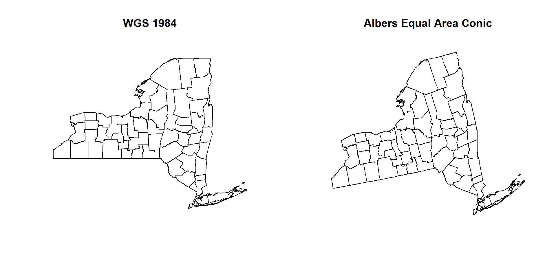
par(mfrow=c(1,1))We can save (write) this file as an ESRI shape with writeOGR() or shapefile() function for future use.
writeOGR(county.PROJ,                         # input spatial data
        dsn=dsn,                              # working directory
        "NY_County_PROJ",                     # output spatial data
        driver="ESRI Shapefile",              # define output as ESRI shape file
      overwrite=TRUE)                         # write on existing file, if exist
# or
shapefile(county.PROJ, paste0(dataFolder,"NY_County_PROJ.shp"),overwrite=TRUE)
Raster Data
This exercise you will learn how to projection transformation of will be done of raster data. In this exercise, we will use SRTM 90 digital Elevation Model New York State which was downloaded from CGIAR-CSI. We will re-project it from WSG84 coordinate to Albers Equal Area Conic NAD83 projection system. In R, you can re-project a single or multiple raster in a batch mode.
Projection of a Single Raster
First, we will re-project one tile of NY DEM raster data (~/NY_DEM_TILES/NY_DEM0.tif) from WGS 1984 CRS to Albers Equal Area Conic projection system. You can load DEM raster in R using raster() function of raster package. If you want to check raster attribute, just simple type r-object name of this raster or use crs() function.
DEM.GCS<-raster(paste0(dataFolder,"Onondaga_DEM.tif"))
DEM.GCS
## class      : RasterLayer
## dimensions : 443, 534, 236562  (nrow, ncol, ncell)
## resolution : 0.001133064, 0.001133064  (x, y)
## extent     : -76.50013, -75.89507, 42.77139, 43.27333  (xmin, xmax, ymin, ymax)
## crs        : +proj=longlat +datum=WGS84 +no_defs +ellps=WGS84 +towgs84=0,0,0
## source     : D:/Dropbox/Spatial Data Analysis and Processing in R/DATA_03/DATA_03/Onondaga_DEM.tif
## names      : Onondaga_DEM
# Or
crs(DEM.GCS)
## CRS arguments:
##  +proj=longlat +datum=WGS84 +no_defs +ellps=WGS84 +towgs84=0,0,0
You notice that CRS of this DEM has already been defined as WGS 84. Now, we will project from WGS 84 to Albers Equal Area Conic NAD83. We will use projectRaster() function with proj.4 projection description of Albers Equal Area Conic NAD83. Be patient, it will take a while to project this DEM data.
DEM.PROJ<-projectRaster(DEM.GCS, crs=usa_albers)
DEM.PROJ
## class : RasterLayer
## dimensions : 526, 695, 365570 (nrow, ncol, ncell)
## resolution : 84.9, 131 (x, y)
## extent : 1476714, 1535720, 480423.3, 549329.3 (xmin, xmax, ymin, ymax)
## crs : +proj=aea +lat_1=20 +lat_2=60 +lat_0=40 +lon_0=-96 +x_0=0 +y_0=0 +datum=NAD83 +units=m +no_defs +ellps=GRS80 +towgs84=0,0,0
## source : memory
## names : Onondaga_DEM
## values : 108.321, 619.3135 (min, max)par(mfrow=c(1,2))
plot(DEM.GCS, main="WGS 1984")
plot(DEM.PROJ, main="Albers Equal Area Conic")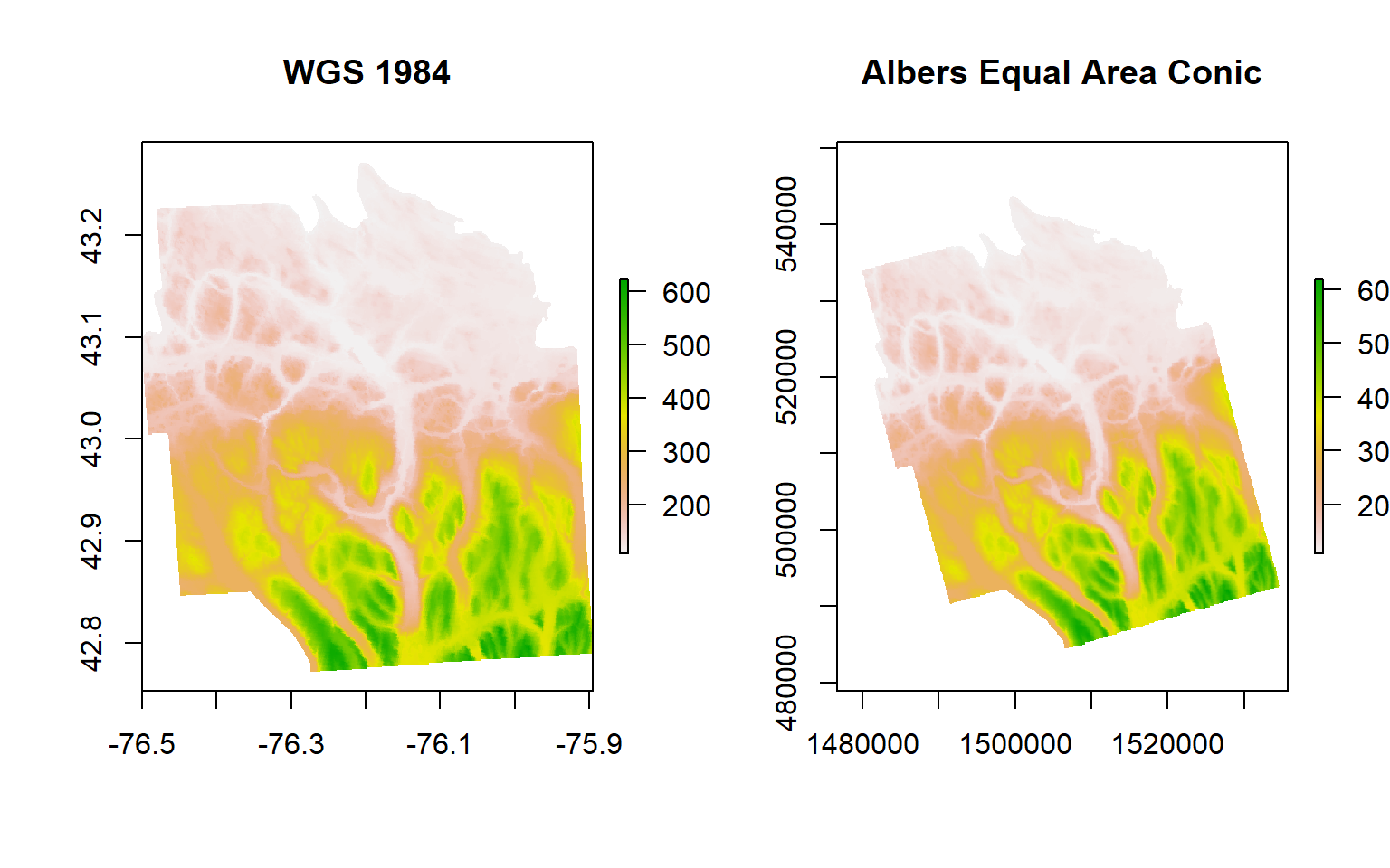
par(mfrow=c(1,1))Now we will save this projected raster using writeRaster() function of raster package
writeRaster(DEM.PROJ,                                      # Input raster
            paste0(dataFolder,"NY_DEM0_PROJ.tiff"),        # output folder and output raster
            "GTiff",                                       # output raster file extension
             overwrite=TRUE)                               # write on existing file, if exist
Batch Projection of Multiple Raster
In this exercise will project four tiles of DEM raster in a loop. First, we will create a list of raster using list.files() function and then will create output raster using gsub() function
# Input raster list
DEM.input <- list.files(path= paste0(dataFolder,".//DEM_TILES"),pattern='.TIF$',full.names=T)
DEM.input
## [1] "D://Dropbox//Spatial Data Analysis and Processing in R//DATA_03//DATA_03//.//DEM_TILES/Onondaga_DEM0.TIF"
## [2] "D://Dropbox//Spatial Data Analysis and Processing in R//DATA_03//DATA_03//.//DEM_TILES/Onondaga_DEM1.TIF"
## [3] "D://Dropbox//Spatial Data Analysis and Processing in R//DATA_03//DATA_03//.//DEM_TILES/Onondaga_DEM2.TIF"
## [4] "D://Dropbox//Spatial Data Analysis and Processing in R//DATA_03//DATA_03//.//DEM_TILES/Onondaga_DEM3.TIF"
# Output raster
DEM.output <- gsub("\\.TIF$", "_PROJ.TIF", DEM.input)
DEM.output
## [1] "D://Dropbox//Spatial Data Analysis and Processing in R//DATA_03//DATA_03//.//DEM_TILES/Onondaga_DEM0_PROJ.TIF"
## [2] "D://Dropbox//Spatial Data Analysis and Processing in R//DATA_03//DATA_03//.//DEM_TILES/Onondaga_DEM1_PROJ.TIF"
## [3] "D://Dropbox//Spatial Data Analysis and Processing in R//DATA_03//DATA_03//.//DEM_TILES/Onondaga_DEM2_PROJ.TIF"
## [4] "D://Dropbox//Spatial Data Analysis and Processing in R//DATA_03//DATA_03//.//DEM_TILES/Onondaga_DEM3_PROJ.TIF"
We will define proj.4 projection description of Albers Equal Area Conic NAD83 as a mew projection and run projectRaster() functioning in a loop
# Define a new projection
newproj <- "+proj=aea +lat_1=29.5 +lat_2=45.5 +lat_0=37.5 +lon_0=-96 +x_0=0 +y_0=0 +datum=NAD83 +units=m +no_defs"
# Reprojection and write raster
for (i in 1:4){
    r <- raster(DEM.input[i])
    PROJ <- projectRaster(r, crs=newproj, method = 'bilinear', filename = DEM.output[i], overwrite=TRUE)
}
rm(list = ls())