5.3.2 DAG-GNN: DAG Structure Learning with Graph Neural Networks
Note: DAG-GNN requires PyTorch . The DAGGNN estimator in pydeepcausalml.discovery learns DAG structure via a VAE-style encoder–decoder with an augmented-Lagrangian acyclicity penalty.
DAG-GNN (Yu et al., ICML 2019) learns the structure of a Directed Acyclic Graph (DAG) from observational data by embedding the problem inside a deep generative model. Where NOTEARS replaces a combinatorial graph search with a smooth optimization over a weighted adjacency matrix \(\mathbf{W}\) , DAG-GNN goes a step further: it wraps that adjacency matrix inside a Variational Autoencoder (VAE) driven by Graph Neural Network (GNN) encoder and decoder modules, so that representation learning and structure learning are trained end-to-end.
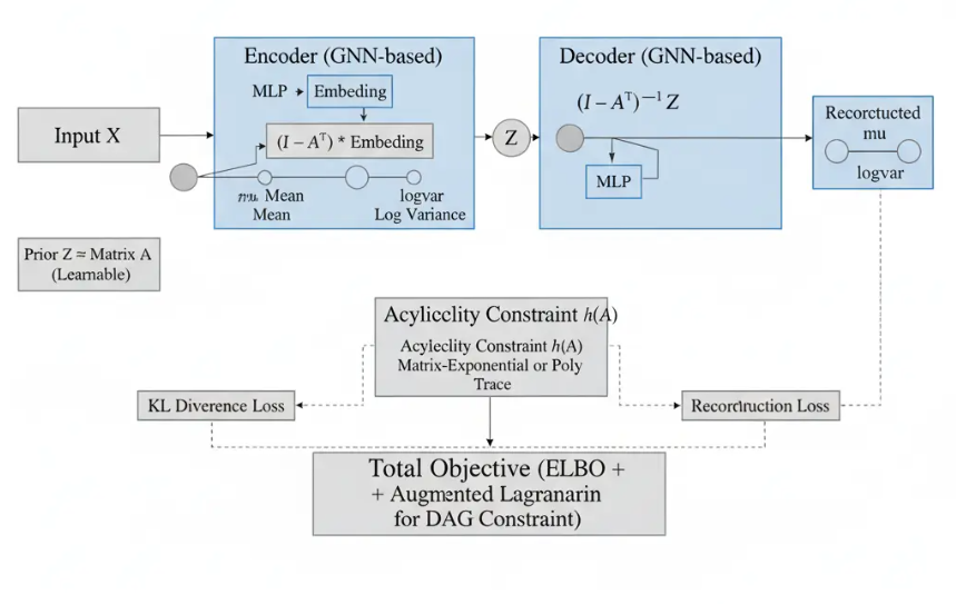
The key insight is that under a linear Structural Equation Model (SEM), \(\mathbf{X} = \mathbf{A}^\top \mathbf{X} + \mathbf{Z}\) , the mapping from noise \(\mathbf{Z}\) to observations \(\mathbf{X}\) is exactly \((\mathbf{I} - \mathbf{A}^\top)^{-1}\mathbf{Z}\) . DAG-GNN makes this causal forward pass the decoder of the VAE, and uses a GNN-filtered MLP as the encoder . The adjacency matrix \(\mathbf{A}\) is a learnable parameter shared between encoder and decoder, so gradient descent simultaneously fits the data and discovers the graph.
Acyclicity is enforced by the same differentiable constraint family as NOTEARS — \(h(\mathbf{A}) = 0\) iff the graph is a DAG — embedded as an augmented Lagrangian penalty in the ELBO objective. This notebook demonstrates the full pipeline: data simulation, model training with stable augmented Lagrangian updates, structure recovery, and downstream causal effect estimation.
Implementation in Python
We use PyDeepCausalML ’s DAGGNN class for causal structure discovery and effect estimation on synthetic data.
Setup
Code
import importlibimport subprocessimport sys= ["numpy" , "pandas" , "scipy" , "torch" , "scikit-learn" ,"matplotlib" , "seaborn" , "networkx" ,for pkg in PACKAGES:= "sklearn" if pkg == "scikit-learn" else pkgtry :except ImportError :"-m" , "pip" , "install" , "-q" , pkg])try :import pydeepcausalml # noqa: F401 except ImportError :"-m" , "pip" , "install" , "-q" ,"git+https://github.com/zia207/PyDeepCausalML.git" ]import pydeepcausalmlprint ("pydeepcausalml" , pydeepcausalml.__version__, "ready." )
pydeepcausalml 0.2.0 ready.
Code
import numpy as npimport pandas as pdimport torchimport matplotlib.pyplot as pltimport seaborn as snsimport networkx as nxfrom sklearn.linear_model import LinearRegressionfrom pydeepcausalml import set_seedfrom pydeepcausalml.metrics import graph_recovery_metrics, shd, peheprint ("torch:" , torch.__version__)print ("cuda:" , torch.cuda.is_available())
torch: 2.12.1+cu130
cuda: False
Code
42 )= True
Data and Data Processing
We generate a small 6-node nonlinear DAG .
Code
def generate_synthetic_dag_data(n_samples= 5000 , n_nodes= 6 , seed= 42 ):= np.random.default_rng(seed)= 3.0 / (n_nodes - 1 ) if n_nodes > 1 else 0.0 = nx.erdos_renyi_graph(n_nodes, p, directed= True , seed= seed)= [(u, v) for u, v in G.edges() if u < v]= nx.DiGraph(edges)= nx.to_numpy_array(G, dtype= float )*= rng.uniform(0.5 , 1.5 , size= A_true.shape)= np.zeros((n_samples, n_nodes))for _ in range (10 ):= rng.standard_normal((n_samples, n_nodes))= np.cos(X @ A_true.T + 1 ) + Z= ((rng.standard_normal(n_samples) + 0.5 * X[:, 0 ] + 0.3 * X[:, 1 ]) > 0 ).astype(float )= 2 * T_var + 0.8 * X[:, 0 ] + np.sin(X[:, 2 ]) + rng.normal(0 , 0.5 , n_samples)4 ] = T_var5 ] = Y_var= [f"X { i} " for i in range (n_nodes)] + ["T" , "Y" ]= pd.DataFrame(np.column_stack([X, T_var, Y_var]), columns= cols)return df, A_true, G= generate_synthetic_dag_data()= synth_dataprint (df.head())= [f"X { i} " for i in range (6 )]= df.copy()= (df[node_cols] - df[node_cols].mean()) / (df[node_cols].std() + 1e-8 )
         X0        X1        X2        X3   X4        X5    T         Y
0  0.004246 -1.327359  2.671251  0.916931  0.0  0.386741  0.0  0.386741
1 -2.385299  0.432979 -0.281234  0.671500  1.0  0.229349  1.0  0.229349
2  0.856719 -1.081930  0.400571 -0.798042  0.0  0.628959  0.0  0.628959
3  0.790588  1.248634  1.301773  1.183922  1.0  3.378329  1.0  3.378329
4 -0.085306 -0.971270 -1.419499  0.624939  0.0 -1.010660  0.0 -1.010660
Data split
Code
= np.random.default_rng(42 )= rng.permutation(len (df_norm))= idx[: int (0.7 * len (idx))]= idx[int (0.7 * len (idx)) :]= temp_idx[: len (temp_idx) // 2 ]= temp_idx[len (temp_idx) // 2 :]= df_norm.iloc[train_idx].reset_index(drop= True )= df_norm.iloc[valid_idx].reset_index(drop= True )= df_norm.iloc[test_idx].reset_index(drop= True )= train_df[node_cols].values.astype(np.float32)= valid_df[node_cols].values.astype(np.float32)= test_df[node_cols].values.astype(np.float32)print ("Train:" , X_train.shape, "Valid:" , X_valid.shape, "Test:" , X_test.shape)
Train: (3500, 6) Valid: (750, 6) Test: (750, 6)
DAG-GNN Model Architecture
DAG-GNN frames causal structure learning as a Variational Autoencoder (VAE) whose latent space is organized by a learnable adjacency matrix \(\mathbf{A}\) .
Acyclicity Constraint \(h(\mathbf{A})\)
Acyclicity is enforced via the NOTEARS-style penalty embedded in the training objective.
Total Objective
\[\mathcal{L} = \text{reconstruction} + \lambda\, h(\mathbf{A})^2 + \text{sparsity}\]
Model instantiation and training
Code
from pydeepcausalml.discovery import DAGGNN42 )= DAGGNN(hidden= 64 , latent= 16 , lambda_dag= 0.1 , epochs= 600 , lr= 1e-3 , random_state= 42 )= model.adjacency_matrix()= 0.10 = (A_learned > threshold).astype(int )print (f"A_eff: min= { A_learned. min ():.4f} , max= { A_learned. max ():.4f} " )print (f"Edges (threshold { threshold} ): { int (A_binary.sum ())} " )
A_eff: min=0.0000, max=0.3787
Edges (threshold 0.1): 30
ATE and CATE Estimation
Code
= ["X0" , "X1" , "X2" , "X3" ]= train_df[cov_cols].values= test_df[cov_cols].values= train_df["T" ].values= test_df["T" ].values= train_df["Y" ].values= test_df["Y" ].values= treatment_train.astype(float )= treatment_test.astype(float )= np.column_stack([treatment_train_bin, X_train_cov])= LinearRegression().fit(X_tr, y_train)= lr_model.coef_[0 ]= np.full(len (y_test), cate_coef)= cate_arr.mean()= 2.0 = np.sqrt(np.mean((y_test - lr_model.predict(np.column_stack([treatment_test_bin, X_test_cov]))) ** 2 ) / len (y_test))= ate_val - 1.96 * se_ate, ate_val + 1.96 * se_ateprint ("=== ATE on test set ===" )print (f"Estimated ATE (true ATE = { true_ate} ): { ate_val:.4f} " )print (f"ATE 95% CI: [ { ci_lb:.4f} , { ci_ub:.4f} ]" )print (f"PEHE: { pehe(true_ate, cate_arr):.4f} " )
=== ATE on test set ===
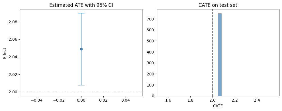
Estimated ATE (true ATE = 2.0): 2.0488
ATE 95% CI: [2.0079, 2.0897]
PEHE: 0.0488
Results visualization
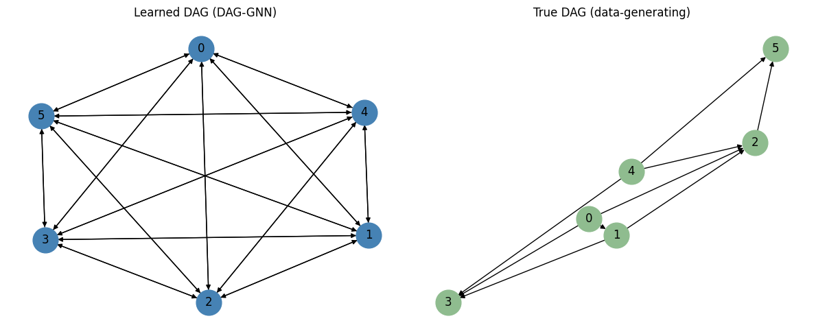
True vs learned DAG
Code
= [f"X { i} " for i in range (6 )]= (A_true != 0 ).astype(int )= plt.subplots(1 , 2 , figsize= (12 , 5 ))for ax, B, title, color in [0 ], A_binary, "Learned DAG (DAG-GNN)" , "steelblue" ),1 ], A_true_bin, "True DAG (data-generating)" , "darkseagreen" ),= nx.from_numpy_array(B, create_using= nx.DiGraph)= nx.spring_layout(G, seed= 42 )= ax, with_labels= True , node_color= color, node_size= 700 , arrows= True )
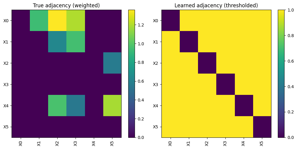
Adjacency matrices: true vs learned
Code
= plt.subplots(1 , 2 , figsize= (10 , 5 ))for ax, M, title in [0 ], A_true, "True adjacency (weighted)" ),1 ], A_binary, "Learned adjacency (thresholded)" ),= ax.imshow(M, cmap= "viridis" , aspect= "auto" )range (6 ), node_labels, rotation= 90 )range (6 ), node_labels)= ax)
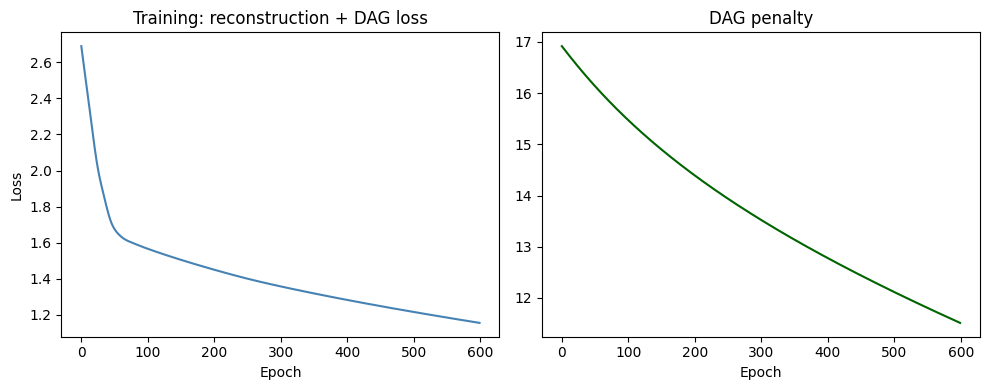
Training curves
Code
= model.history_if hist.get("loss" ):= plt.subplots(1 , 2 , figsize= (10 , 4 ))0 ].plot(hist["loss" ], color= "steelblue" )0 ].set_title("Training: reconstruction + DAG loss" )0 ].set_xlabel("Epoch" )0 ].set_ylabel("Loss" )if hist.get("dag" ):1 ].plot(hist["dag" ], color= "darkgreen" )1 ].set_title("DAG penalty" )1 ].set_xlabel("Epoch" )
ATE and CATE summary
Code
= plt.subplots(1 , 2 , figsize= (10 , 4 ))0 ].errorbar([0 ], [ate_val], yerr= [[ate_val - ci_lb], [ci_ub - ate_val]], fmt= "o" , color= "steelblue" , capsize= 8 )0 ].axhline(true_ate, color= "gray" , linestyle= "--" )0 ].set_title("Estimated ATE with 95% CI" )0 ].set_ylabel("Effect" )1 ].hist(cate_arr, bins= 30 , color= "steelblue" , alpha= 0.7 )1 ].axvline(true_ate, color= "gray" , linestyle= "--" )1 ].set_title("CATE on test set" )1 ].set_xlabel("CATE" )
Summary and conclusion
DAG-GNN turns the notoriously hard DAG-learning problem into a differentiable VAE + GNN optimization using PyDeepCausalML ’s DAGGNN estimator.
Run DAG-GNN on your observational dataset.
Threshold the learned adjacency (default 0.10 ) to obtain a sparse causal DAG.
Feed the DAG into downstream effect estimators for ATE/CATE analysis.