5.2.4 Causal Generative Network (CausalGAN)

Note: CausalGAN requires PyTorch. The CausalGAN estimator in pydeepcausalml.generative trains structural equation generators with per-node labellers on a user-specified causal DAG.

Causal Generative Network (CausalGAN) is a causal-aware extension of the classic GAN framework, introduced by Kocaoglu et al. (2018) in the paper CausalGAN: Learning Causal Implicit Generative Models with Adversarial Training. It lets you train a generative model that respects a user-specified causal DAG while still producing high-quality, realistic samples from the joint distribution. The key advantage is that the model can answer causal queries, interventions ($\mathrm{do}(\cdot)$) and counterfactuals, without any retraining or additional data, something a vanilla GAN cannot do.

Why Standard GANs Fall Short

A normal GAN (Goodfellow et al., 2014) learns an implicit generator $G$ that maps noise $Z \sim p_Z$ to samples $\hat{\mathbf{v}} = G(Z)$ so that the joint distribution $p(\hat{X}, \hat{T}, \hat{Y})$ matches the data distribution $p(X, T, Y)$. However, because the generator is a black-box neural network, it has no notion of causal mechanisms.

You cannot ask it:

Interventional query: “What would $Y$ be if we forced $T = 1$ for everyone?” ($\mathbb{E}[Y \mid \mathrm{do}(T=1)]$).
Counterfactual query: “Given that this patient had $T=0$ and outcome $Y=0$, what would their $Y$ have been if they had received treatment $T=1$?”

CausalGAN fixes this by turning the generator into a Structural Causal Model (SCM) whose functional form is exactly the causal graph you provide.

How CausalGAN Works

1. Structural Equation Generators (The Core Architecture)

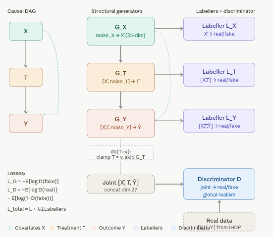
Architecturally, CausalGAN decomposes the generator into separate modules that mirror the structure of the causal DAG. For a simple DAG with $X \to T \to Y$ and $X \to Y$, the generator is structured as follows:

Instead of one monolithic generator, CausalGAN decomposes the generator according to the topological order of the DAG. Every node $V_i$ gets its own sub-generator $G_i$:

\[ \begin{align*} \hat{X} &= G_X(Z_X) \\ \hat{T} &= G_T(\hat{X}, Z_T) \\ \hat{Y} &= G_Y(\hat{X}, \hat{T}, Z_Y) \end{align*} \]

$Z_X, Z_T, Z_Y \sim \mathcal{N}(0, I)$ are independent exogenous noise vectors (the “unobserved confounders” in the SCM).
Each $G_i$ is a neural network (typically MLPs or CNNs depending on the domain) that takes:
- The generated values of its causal parents (already sampled upstream), and
- Its own private noise.
Data flow is strictly causal: a child never “sees” its descendants. This exactly implements the structural equations of a causal DAG:

$ V_i := f_i((V_i), U_i), U_i !!! $$

Because the architecture hard-wires the graph, the generatorautomatically satisfies the Markov factorization of the joint distribution induced by the DAG.

2. Interventions via Clamping (Do-Calculus in One Line)

To perform an intervention $\mathrm{do}(T = t)$:

Skip $G_T$ entirely.
Set $\hat{T} \leftarrow t$ (a constant).
Feed the clamped $\hat{T}$ into all downstream generators ($G_Y$ in the example).

\[ \hat{Y}_{\mathrm{do}(T=1)} = G_Y(\hat{X}, \hat{T}=1, Z_Y) \]

No weights are changed. This is exactly Pearl’s $\mathrm{do}$-operator realized inside the generator. You can now compute interventional quantities by sampling many such trajectories and averaging (e.g., average treatment effect, conditional interventions, etc.).

3. Labeller Networks (The Key Training Innovation)

Standard GANs only have one global discriminator $D$ that tries to distinguish real $(X,T,Y)$ from fake $(\hat{X},\hat{T},\hat{Y})$. CausalGAN adds one small “labeller” (local discriminator/classifier) per node.

Global discriminator $D_{\text{joint}}$: ensures the entire joint looks realistic.
Node-specific labellers $D_i$: each $D_i$ is trained to distinguish the marginal/conditional distribution of node $i$ given its parents in both real and generated data.

The total adversarial loss becomes:

\[ \mathcal{L} = \mathcal{L}_{\text{joint}} + \sum_i \lambda_i \mathcal{L}_{\text{label},i} \]

This extra supervision forces each structural equation $G_i$ to match the correct conditional $p(V_i \mid \text{Pa}(V_i))$ implied by the data. Without labellers, a plain GAN could learn a joint that is statistically close but violates the causal conditionals.

4. Counterfactual Abduction (Answering “What if this specific patient had been treated?”)

Counterfactuals require three steps (abduction → action → prediction), exactly as in Pearl’s SCM framework:

Abduction: Given a real observation $(x, t, y)$, find the noise realization $\mathbf{u}^* = (u_X^*, u_T^*, u_Y^*)$ that best explains it:

\[ \mathbf{u}^* = \arg\min_{\mathbf{u}} \;\; \bigl\| G(\mathbf{u}) - (x,t,y) \bigr\|_2^2 + \text{regularizers} \] This is solved by gradient descent on the noise vectors (a few dozen steps at inference time; no retraining).

Action: Apply the intervention by clamping the desired variable (e.g., set $\hat{T} = 1$).
Prediction: Re-run the generator with the same noise $\mathbf{u}^*$ but the new intervention:

\[ y_{\text{CF}} = G_Y(x, \hat{T}=1, u_Y^*) \]

Because the noises are held fixed, you are answering “what would this exact individual have experienced under the counterfactual treatment?”—the purest form of individual-level causal reasoning.

Advantages and Practical Notes

Zero extra training cost for causal queries: once trained, any intervention or counterfactual is a simple forward pass (or a short abduction optimization).
Works with any differentiable generator (MLPs, CNNs, transformers, etc.).
Scalable: the number of extra labellers is linear in the number of nodes, and each is tiny.
Applications: medical imaging (what-if different treatments?), fairness (counterfactual fairness auditing), causal data augmentation, policy evaluation, etc.

In short, CausalGAN is the first practical way to turn a black-box generative model into a white-box Structural Causal Model that obeys both statistical realism and the causal graph you care about. The combination of structural-equation generators, per-node labellers, and explicit noise abduction gives you full do-calculus and counterfactual power inside the adversarial training loop.

Implementation in Python

We fit CausalGAN with pydeepcausalml.generative.CausalGAN on IHDP.

Check and Install Required Python Packages

The following packages are used in this notebook. Install any missing packages with the cell below:

numpy, pandas, scipy, torch, scikit-learn, matplotlib, seaborn, pydeepcausalml

Code

import importlib
import subprocess
import sys

PACKAGES = [
    "numpy", "pandas", "scipy", "torch", "scikit-learn",
    "matplotlib", "seaborn",
]

for pkg in PACKAGES:
    mod = "sklearn" if pkg == "scikit-learn" else pkg
    try:
        importlib.import_module(mod)
    except ImportError:
        subprocess.check_call([sys.executable, "-m", "pip", "install", "-q", pkg])

try:
    import pydeepcausalml  # noqa: F401
except ImportError:
    subprocess.check_call(
        [sys.executable, "-m", "pip", "install", "-q",
         "git+https://github.com/zia207/PyDeepCausalML.git"]
    )

import pydeepcausalml
print("pydeepcausalml", pydeepcausalml.__version__, "ready.")

pydeepcausalml 0.2.0 ready.

Verify imports

Code

import numpy as np
import pandas as pd
import torch
import matplotlib.pyplot as plt
import seaborn as sns
from pydeepcausalml import set_seed

print("torch:", torch.__version__)
print("cuda:", torch.cuda.is_available())

torch: 2.12.1+cu130
cuda: False

Code

set_seed(42)
run_fast = True

Load and preprocess IHDP

Data loading and preprocessing

IHDP is small per replication (~6.7k rows after merging the nine NPCI CSVs). Setting replications=100 stacks 100 copies for Monte Carlo–style benchmarks but needs large RAM and can stress the machine; this tutorial defaults to replications=1.

The next cell defines Z_train, Z_test (needed for Z_test_t in training), Z_test_eval (float64 copy for metrics), and cols.

Code

def load_ihdp(replications: int = 2, random_state: int = 1):
    """Load IHDP semi-synthetic benchmark (CausalML format)."""
    base_url = "https://raw.githubusercontent.com/uber/causalml/master/docs/examples/data"
    cols = ["treatment", "y_factual", "y_cfactual", "mu0", "mu1"] + [f"X{i}" for i in range(25)]
    parts = []
    for i in range(1, 10):
        url = f"{base_url}/ihdp_npci_{i}.csv"
        tmp = pd.read_csv(url, header=None)
        tmp.columns = cols[: tmp.shape[1]]
        parts.append(tmp)
    df = pd.concat(parts, ignore_index=True)
    if replications > 1:
        df = pd.concat([df] * replications, ignore_index=True)
    perm = list(range(6, 25)) + list(range(6))
    xcols = [f"X{i}" for i in range(25)]
    X = df[xcols].to_numpy(dtype=float)[:, perm]
    treatment = df["treatment"].to_numpy(dtype=int)
    y = df["y_factual"].to_numpy(dtype=float)
    mu0 = df["mu0"].to_numpy(dtype=float)
    mu1 = df["mu1"].to_numpy(dtype=float)
    tau = np.where(
        treatment == 1,
        df["y_factual"] - df["y_cfactual"],
        df["y_cfactual"] - df["y_factual"],
    )
    n = len(X)
    rng = np.random.default_rng(random_state)
    val_idx = rng.choice(n, size=int(0.2 * n), replace=False)
    train_idx = np.setdiff1d(np.arange(n), val_idx)
    return df, X, treatment, y, tau, mu0, mu1, train_idx, val_idx


def preprocess_ihdp_features(train_x, test_x, cont_cols=None):
    """Scale continuous covariates (cols 19–24 after binary-first permutation)."""
    cont_cols = cont_cols or list(range(19, 25))
    train = train_x.copy()
    test = test_x.copy()
    means = train[:, cont_cols].mean(axis=0)
    sds = train[:, cont_cols].std(axis=0)
    sds[sds == 0] = 1.0
    train[:, cont_cols] = (train[:, cont_cols] - means) / sds
    test[:, cont_cols] = (test[:, cont_cols] - means) / sds
    return train, test


def synthetic_ihdp_fallback(n=5000, p=25, random_state=42):
    rng = np.random.default_rng(random_state)
    X = rng.normal(size=(n, p))
    lin = 0.3 * X[:, 0] - 0.2 * X[:, 1] + 0.15 * X[:, 2]
    tau = 0.5 + 0.2 * np.tanh(X[:, 4])
    mu0 = lin + 0.1 * X[:, 6] ** 2
    mu1 = mu0 + tau
    ps = 1 / (1 + np.exp(-(0.2 * X[:, 0] - 0.1 * X[:, 1])))
    t = rng.binomial(1, ps)
    y = np.where(t == 1, mu1, mu0) + rng.normal(scale=1.0, size=n)
    perm = list(range(6, 25)) + list(range(6))
    return X[:, perm], t, y, mu0, mu1, tau

try:
    _, X, treatment, y, tau, mu0, mu1, train_idx, val_idx = load_ihdp(replications=1)
except Exception:
    X, treatment, y, mu0, mu1, tau = synthetic_ihdp_fallback()
    n = len(X)
    rng = np.random.default_rng(42)
    train_idx = rng.choice(n, size=int(0.8 * n), replace=False)
    val_idx = np.setdiff1d(np.arange(n), train_idx)

X_train, X_test = X[train_idx], X[val_idx]
t_train, t_test = treatment[train_idx], treatment[val_idx]
y_train = y[train_idx]
tau_test = mu1[val_idx] - mu0[val_idx]

# Scale first 6 continuous columns (original X0-X5; after perm they are cols 19-24)
cont = list(range(19, 25))
means = X_train[:, cont].mean(0)
sds = X_train[:, cont].std(0)
sds[sds == 0] = 1
X_train[:, cont] = (X_train[:, cont] - means) / sds
X_test[:, cont] = (X_test[:, cont] - means) / sds

rng = np.random.default_rng(42)
sub = rng.choice(len(X_train), size=min(5000, len(X_train)), replace=False)
X_tr, t_tr, y_tr = X_train[sub], t_train[sub], y_train[sub]
print("Train:", X_tr.shape, "| Test:", X_test.shape)

Train: (5000, 25) | Test: (1344, 25)

Fit CausalGAN

Code

from pydeepcausalml.generative import CausalGAN

cg = CausalGAN(
    hidden=64 if run_fast else 128,
    noise_dim=8,
    lambda_lab=0.5,
    epochs=150 if run_fast else 300,
    batch_size=256,
    lr=1e-3,
    random_state=42,
    verbose=True,
    log_every=10,
)
cg.fit(X_tr, t_tr, y_tr)

CausalGAN(epochs=150, lr=0.001, batch_size=256, weight_decay=0.0001, early_stopping_patience=None, device=None)

Interventional ATE via do(T)

We estimate the ATE by clamping the treatment node to $do(T=1)$ versus $do(T=0)$ and averaging the difference in generated outcomes across the test set. Because the generator is stochastic, we average over n_samples draws to reduce Monte-Carlo noise.

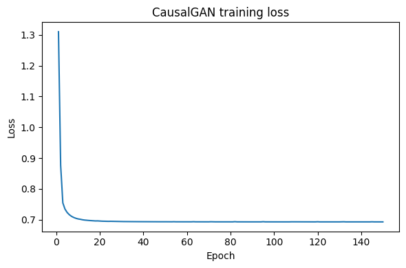
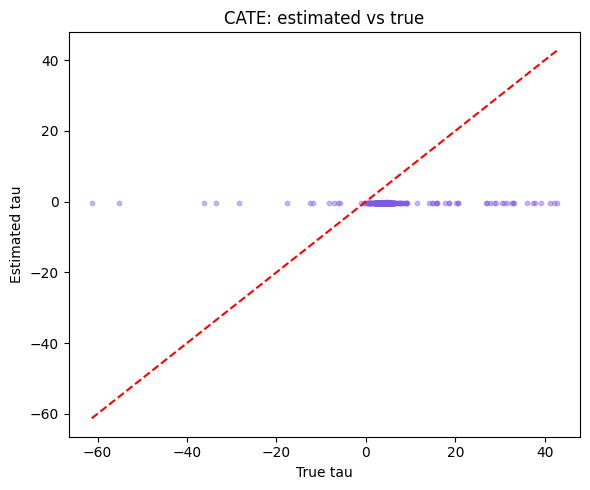
A note on GAN stability. Adversarial causal estimators are markedly harder to train than the VAE- and SCM-based models elsewhere in this series. The min–max objective offers no single loss to watch for convergence, and on heavy-tailed semi-synthetic benchmarks such as IHDP the generator often captures the shape of the effect better than its magnitude. Read the estimate below as indicative, and compare it against the DSCM and CausalEGM notebooks — which target the same IHDP outcome and are usually better calibrated — before drawing conclusions.

Code

ate_gen = cg.predict_cate(X_test, n_samples=100).mean()
ate_true = tau_test.mean()
print(f"Estimated ATE (do-calculus): {ate_gen:.4f}")
print(f"True ATE: {ate_true:.4f}")

Estimated ATE (do-calculus): -0.2754
True ATE: 4.9491

CATE PEHE on test set

Code

ite_hat = cg.predict_cate(X_test, n_samples=50)
pehe = np.sqrt(np.mean((ite_hat - tau_test) ** 2))
print(f"sqrt(PEHE): {pehe:.4f}")
print(f"Std of true tau: {tau_test.std():.4f}")

sqrt(PEHE): 10.3721
Std of true tau: 8.9599

Training loss and ITE scatter

Code

hist = cg.history_
if hist.get("loss"):
    plt.figure(figsize=(6, 4))
    plt.plot(range(1, len(hist["loss"]) + 1), hist["loss"])
    plt.xlabel("Epoch")
    plt.ylabel("Loss")
    plt.title("CausalGAN training loss")
    plt.tight_layout()
    plt.show()

plt.figure(figsize=(6, 5))
n_sc = min(500, len(X_test))
plt.scatter(tau_test[:n_sc], ite_hat[:n_sc], alpha=0.4, s=10, color="#7b5ce0")
mn = min(tau_test[:n_sc].min(), ite_hat[:n_sc].min())
mx = max(tau_test[:n_sc].max(), ite_hat[:n_sc].max())
plt.plot([mn, mx], [mn, mx], "r--")
plt.xlabel("True tau")
plt.ylabel("Estimated tau")
plt.title("CATE: estimated vs true")
plt.tight_layout()
plt.show()

Summary and Conclusions

This tutorial demonstrated how to implement and evaluate a Causal Generative Adversarial Network (CausalGAN) in Python using the pydeepcausalml package. We covered: - Building structural equation generators that respect a user-specified causal graph. - Performing interventional analysis by clamping treatment variables. - Conducting counterfactual inference through abduction-action-prediction. - Evaluating model performance using metrics like FID-proxy, SEM R², and CATE PEHE.

When to reach for CausalGAN. Its strength is generative — sampling whole counterfactual outcomes while respecting a user-specified structural graph — rather than producing the tightest ATE on a benchmark. For point estimation on tabular data, DSCM, CausalEGM, or CausalDiscrepancyVAE are usually more stable and better calibrated. Reach for CausalGAN when you need to generate plausible interventional or counterfactual samples, not merely summarize an average effect.

Resources

Kocaoglu et al. (2018). “CausalGAN: Learning Causal Implicit Generative Models with Adversarial Training.arXiv:1709.02023
{CausalML} package documentation: https://docs.uber.com/causal ml/