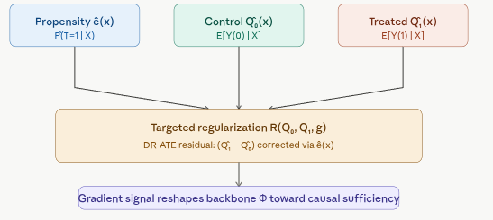
from pathlib import Path
import os
import numpy as np
import pandas as pd
from sklearn.ensemble import RandomForestRegressor
from sklearn.linear_model import ElasticNet, LogisticRegression, LinearRegression
from sklearn.model_selection import KFold


def load_nsw_mixtape() -> pd.DataFrame:
    """Load NSW (Lalonde) mixtape data (same variables as causaldata::nsw_mixtape)."""
    try:
        import causaldata.nsw_mixtape.data as nsw_data
        dta = Path(nsw_data.__file__).parent / "nsw_mixtape.dta"
        return pd.read_stata(dta)
    except Exception:
        pass
    url = (
        "https://raw.githubusercontent.com/NickCH-K/causaldata/master/"
        "data-raw/nsw_mixtape.dta"
    )
    return pd.read_stata(url)


def propensity_elastic_net(X: np.ndarray, treatment: np.ndarray) -> np.ndarray:
    model = LogisticRegression(
        penalty="elasticnet", solver="saga", l1_ratio=0.5, max_iter=2000
    )
    model.fit(X, treatment)
    return model.predict_proba(X)[:, 1]


class SLearner:
    def __init__(self, learner: str = "ranger"):
        self.learner = learner

    def fit(self, X, t, y):
        Xt = np.column_stack([X, t])
        if self.learner == "lm":
            self.model_ = LinearRegression().fit(Xt, y)
        else:
            self.model_ = RandomForestRegressor(
                n_estimators=100, random_state=42, n_jobs=-1
            ).fit(Xt, y)
        return self

    def predict(self, X):
        y0 = self.model_.predict(np.column_stack([X, np.zeros(len(X))]))
        y1 = self.model_.predict(np.column_stack([X, np.ones(len(X))]))
        return y1 - y0


class TLearner:
    def __init__(self, learner: str = "ranger"):
        self.learner = learner

    def fit(self, X, t, y):
        t = t.astype(int)
        if self.learner == "lm":
            self.m0_ = LinearRegression().fit(X[t == 0], y[t == 0])
            self.m1_ = LinearRegression().fit(X[t == 1], y[t == 1])
        else:
            self.m0_ = RandomForestRegressor(
                n_estimators=100, random_state=42, n_jobs=-1
            ).fit(X[t == 0], y[t == 0])
            self.m1_ = RandomForestRegressor(
                n_estimators=100, random_state=42, n_jobs=-1
            ).fit(X[t == 1], y[t == 1])
        return self

    def predict(self, X):
        return self.m1_.predict(X) - self.m0_.predict(X)


class XLearner:
    def __init__(self, learner: str = "ranger"):
        self.learner = learner

    def _reg(self):
        if self.learner == "lm":
            return LinearRegression()
        return RandomForestRegressor(n_estimators=100, random_state=42, n_jobs=-1)

    def fit(self, X, t, y, p=None):
        t = t.astype(int)
        p = propensity_elastic_net(X, t) if p is None else p
        m0, m1 = self._reg(), self._reg()
        m0.fit(X[t == 0], y[t == 0])
        m1.fit(X[t == 1], y[t == 1])
        d1 = y[t == 1] - m0.predict(X[t == 1])
        d0 = m1.predict(X[t == 0]) - y[t == 0]
        tau1 = self._reg().fit(X[t == 1], d1)
        tau0 = self._reg().fit(X[t == 0], d0)
        self.p_, self.tau0_, self.tau1_ = p, tau0, tau1
        return self

    def predict(self, X):
        return self.p_ * self.tau0_.predict(X) + (1 - self.p_) * self.tau1_.predict(X)


class RLearner:
    def __init__(self, learner: str = "ranger", n_fold: int = 3):
        self.learner = learner
        self.n_fold = n_fold

    def _reg(self):
        if self.learner == "lm":
            return LinearRegression()
        return RandomForestRegressor(n_estimators=100, random_state=42, n_jobs=-1)

    def fit(self, X, t, y, p=None):
        t = t.astype(int).astype(float)
        p = propensity_elastic_net(X, t) if p is None else p
        e = t - p
        m = self._reg()
        kf = KFold(n_splits=self.n_fold, shuffle=True, random_state=42)
        y_hat = np.zeros_like(y, dtype=float)
        for tr, va in kf.split(X):
            m.fit(X[tr], y[tr])
            y_hat[va] = m.predict(X[va])
        resid = y - y_hat
        tau = self._reg()
        tau.fit(X, resid / (e + 1e-6), sample_weight=e**2)
        self.tau_ = tau
        return self

    def predict(self, X):
        return self.tau_.predict(X)


def get_cumgain(df_preds, outcome_col="y", treatment_col="w", treatment_effect_col="tau", normalize=True):
    """Cumulative gain curve (CausalML-style AUUC helper)."""
    y = df_preds[outcome_col].to_numpy()
    w = df_preds[treatment_col].to_numpy()
    tau = df_preds[treatment_effect_col].to_numpy()
    model_cols = [c for c in df_preds.columns if c not in {outcome_col, treatment_col, treatment_effect_col}]
    n = len(df_preds)
    out = {}
    for col in model_cols:
        scores = df_preds[col].to_numpy()
        order = np.argsort(-scores)
        cum = []
        treated_so_far = control_so_far = 0.0
        for i, idx in enumerate(order, start=1):
            if w[idx] == 1:
                treated_so_far += y[idx]
            else:
                control_so_far += y[idx]
            lift = treated_so_far / max((w[order[:i]] == 1).sum(), 1) - control_so_far / max(
                (w[order[:i]] == 0).sum(), 1
            )
            cum.append(lift)
        curve = np.array(cum)
        if normalize and curve[-1] != 0:
            curve = curve / np.abs(curve[-1])
        out[col] = curve
    out[treatment_effect_col] = out.get(treatment_effect_col, out[model_cols[0]])
    return pd.DataFrame(out)


def plot_gain(df_preds, outcome_col="y", treatment_col="w", treatment_effect_col="tau", model_cols=None, main="", normalize=True):
    import matplotlib.pyplot as plt

    gain = get_cumgain(df_preds, outcome_col, treatment_col, treatment_effect_col, normalize)
    model_cols = model_cols or [c for c in gain.columns]
    plt.figure(figsize=(8, 5))
    for col in model_cols:
        if col in gain.columns:
            plt.plot(gain[col].values, label=col)
    plt.xlabel("Population fraction targeted")
    plt.ylabel("Cumulative gain" + (" (normalized)" if normalize else ""))
    plt.title(main)
    plt.legend()
    plt.tight_layout()
    plt.show()


def load_ihdp(replications: int = 2, random_state: int = 1):
    base_url = "https://raw.githubusercontent.com/uber/causalml/master/docs/examples/data"
    cols = ["treatment", "y_factual", "y_cfactual", "mu0", "mu1"] + [f"X{i}" for i in range(25)]
    parts = []
    for i in range(1, 10):
        url = f"{base_url}/ihdp_npci_{i}.csv"
        tmp = pd.read_csv(url, header=None)
        tmp.columns = cols[: tmp.shape[1]]
        parts.append(tmp)
    df = pd.concat(parts, ignore_index=True)
    if replications > 1:
        df = pd.concat([df] * replications, ignore_index=True)
    binfeats = [f"X{i}" for i in range(6, 25)]
    contfeats = [f"X{i}" for i in range(6)]
    xcols = binfeats + contfeats
    X = df[xcols].to_numpy(dtype=float)
    treatment = df["treatment"].to_numpy(dtype=int)
    y = df["y_factual"].to_numpy(dtype=float)
    tau = np.where(
        treatment == 1,
        df["y_factual"] - df["y_cfactual"],
        df["y_cfactual"] - df["y_factual"],
    )
    n = len(X)
    rng = np.random.default_rng(random_state)
    val_idx = rng.choice(n, size=int(0.2 * n), replace=False)
    train_idx = np.setdiff1d(np.arange(n), val_idx)
    return df, X, treatment, y, tau, train_idx, val_idx


def simulate_hidden_confounder(n=2000, p=5, sigma=1.0, adj=0, random_state=42):
    """Synthetic DGP with latent confounder (CausalML-style benchmark)."""
    rng = np.random.default_rng(random_state)
    z = rng.normal(size=n)
    X = np.column_stack([z + rng.normal(scale=sigma, size=n) for _ in range(p)])
    e = 1 / (1 + np.exp(-(adj + 0.5 * z)))
    w = rng.binomial(1, e)
    b = 2 * z + rng.normal(scale=sigma, size=n)
    tau = 0.5 + 0.3 * z
    y = b + w * tau + rng.normal(scale=sigma, size=n)
    return {"X": X, "y": y, "w": w, "tau": tau, "b": b, "e": e}


def result_table(df_preds, tau_true):
    model_cols = [c for c in ["S", "T", "X", "R", "GANITE", "CEVAE"] if c in df_preds.columns]
    methods = model_cols + ["actual"]
    ate = [df_preds[m].mean() for m in model_cols] + [float(tau_true.mean())]
    mae = [float(np.mean(np.abs(df_preds[m] - tau_true))) for m in model_cols] + [np.nan]
    gain = get_cumgain(df_preds)
    auuc = [float(gain[m].mean()) if m in gain.columns else np.nan for m in model_cols]
    auuc.append(float(gain["tau"].mean()) if "tau" in gain.columns else np.nan)
    return pd.DataFrame({"Method": methods, "ATE": ate, "MAE": mae, "AUUC": auuc})


def synthetic_summary(preds, tau_ref, actual_ate):
    rows = []
    for name, p in preds.items():
        rows.append({
            "Method": name,
            "ATE": p.mean(),
            "MSE": np.mean((p - tau_ref) ** 2),
            "AbsPctErrorATE": abs(p.mean() / actual_ate - 1) if actual_ate != 0 else np.nan,
        })
    rows.append({"Method": "Actuals", "ATE": actual_ate, "MSE": np.nan, "AbsPctErrorATE": np.nan})
    return pd.DataFrame(rows)

from pydeepcausalml.effect import DragonNet

df = load_nsw_mixtape()
y_col, t_col = "re78", "treat"
x_cols = ["age", "educ", "black", "hisp", "marr", "nodegree", "re74", "re75"]
df = df.dropna(subset=[y_col, t_col] + x_cols).copy()
df[t_col] = df[t_col].astype(int)

X = df[x_cols].to_numpy(dtype=float)
X = (X - X.mean(axis=0)) / (X.std(axis=0) + 1e-8)
t_vec = df[t_col].to_numpy(dtype=int)
y_vec = df[y_col].to_numpy(dtype=float)
print("Sample size:", len(X), "| Covariates:", X.shape[1])