Python Banner

5.1.5 NeuralDML: Neural Double Machine Learning for the Average Treatment Effect

Neural Double Machine Learning (NeuralDML) estimates the average treatment effect (ATE) under a partially linear causal model by combining cross-fitted nuisance regression with residual-on-residual identification (Chernozhukov, Chetverikov, Demirer, Duflo, Hansen, Newey & Robins, 2018). Unlike ITE-focused architectures such as TARNet or GANITE, NeuralDML targets a single scalar causal quantity — the population-average effect of treatment — and accompanies the point estimate with a heteroskedasticity-robust confidence interval suitable for inference.

Overview

Observational causal inference from high-dimensional covariates requires two things simultaneously: flexible models for nuisance functions (outcome and propensity) and valid statistical inference for the causal parameter. Classical parametric regression fails when the relationship between covariates and outcomes is nonlinear. Pure deep learning (TARNet, DragonNet) can capture nonlinearity but typically returns point ITE predictions without principled uncertainty quantification for the ATE.

Double/debiased machine learning (DML) resolves this tension. Under the partially linear model

\[Y = \theta T + g(X) + \varepsilon, \qquad T = e(X) + \nu,\]

where \(g(X) = \mathbb{E}[Y \mid X]\) and \(e(X) = \mathbb{E}[T \mid X]\), the ATE \(\theta\) is identified as the coefficient in a regression of outcome residuals on treatment residuals:

\[\tilde{Y}_i = Y_i - \hat{m}(X_i), \qquad \tilde{T}_i = T_i - \hat{e}(X_i)\]

\[\hat{\theta} = \frac{\sum_i \tilde{T}_i \, \tilde{Y}_i}{\sum_i \tilde{T}_i^2}\]

NeuralDML in PyDeepCausalML implements this pipeline with MLP nuisance learners and K-fold cross-fitting to avoid overfitting bias from using the same data to estimate nuisances and the treatment effect.

The cross-fitting pipeline

Cross-fitting is the key ingredient that makes DML statistically valid with flexible machine learning. Without it, reusing the same observations to fit \(\hat{m}\) and \(\hat{e}\) and then to estimate \(\theta\) introduces regularization bias that does not vanish with sample size.

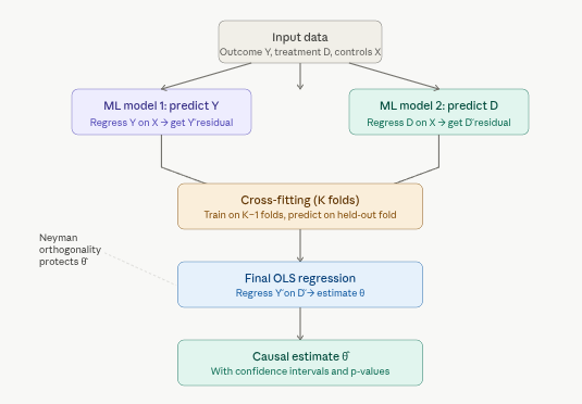
The diagram below shows the standard DML workflow: partition the data, fit nuisances on training folds, compute out-of-sample residuals on held-out folds, then aggregate.

Step 1: Cross-fitting. Split the data into \(K \ge 2\) folds. For each fold \(k\), train the outcome nuisance \(\hat{m}^{(-k)}\) and propensity nuisance \(\hat{e}^{(-k)}\) on all data except fold \(k\).

Step 2: Residualization. For observations in fold \(k\), compute out-of-sample residuals \(\tilde{Y}_i = Y_i - \hat{m}^{(-k)}(X_i)\) and \(\tilde{T}_i = T_i - \hat{e}^{(-k)}(X_i)\).

Step 3: ATE estimation. Regress \(\tilde{Y}\) on \(\tilde{T}\) (no intercept) to obtain \(\hat{\theta}\), the cross-fitted ATE.

Step 4: Inference. Construct a heteroskedasticity-robust (sandwich) standard error from the influence functions \(\psi_i = \tilde{T}_i(\tilde{Y}_i - \hat{\theta}\,\tilde{T}_i)\) and form a normal-approximation confidence interval.

Neural nuisance learners

In classical DML, \(\hat{m}\) and \(\hat{e}\) are often random forests or lasso regressions. NeuralDML replaces both with shared-architecture MLPs:

• Outcome model \(\hat{m}(X)\): MLP with MSE loss, predicting \(\mathbb{E}[Y \mid X]\).
• Propensity model \(\hat{e}(X)\): MLP with BCE loss, predicting \(\mathbb{P}(T=1 \mid X)\) via a sigmoid output.

Both networks use the same hidden-layer specification (hidden=(64, 64) by default) and are trained with Adam for epochs iterations per fold. Covariates and outcomes are standardized internally for stable optimization; the final ATE is rescaled to the original outcome units.

The partially linear structure means NeuralDML assumes a constant treatment effect — it cannot recover heterogeneous ITE profiles. In exchange, it provides Neyman-orthogonal estimation: the ATE estimate is insensitive to first-order errors in the nuisance functions, and the confidence interval is asymptotically valid under standard regularity conditions.

Relationship to other methods

Method	Target	Heterogeneous effects	Uncertainty (ATE)	Nuisance modeling	Cross-fitting
S/T/X/R Learners	ITE → ATE	Yes	No (bootstrap needed)	Flexible (RF, LM)	Optional
TARNet	ITE → ATE	Yes	No	Deep (shared + heads)	No
DragonNet	ITE → ATE	Yes	No	Deep (3-headed)	No
NeuralDML	ATE	No (constant θ)	Yes (robust SE)	Deep (MLP)	Yes (required)
GANITE	ITE	Yes	Yes (generative)	GAN	No

Choose NeuralDML when the research question is “What is the average effect of treatment, and can I report a confidence interval?” rather than “Which individuals benefit most?”

Assumptions and limitations

Assumptions: - Unconfoundedness: \(T \perp (Y(0), Y(1)) \mid X\) — all confounders are observed in \(X\). - Partially linear model: the treatment effect is constant (homogeneous) across covariate values. - Overlap: propensity scores are bounded away from 0 and 1. - Cross-fitting: at least 2 folds (n_splits >= 2) for valid inference.

Limitations: - Cannot estimate individual treatment effects or treatment effect heterogeneity. - Inference relies on the partially linear specification; if the true effect varies strongly with \(X\), the ATE is still well-defined but may not summarize heterogeneity meaningfully. - Neural nuisance learners require tuning (epochs, hidden, lr) like any deep model. - Normal-approximation CIs assume sufficient sample size; small-\(n\) settings may need bootstrap alternatives.

Implementation in Python

We implement NeuralDML with PyDeepCausalML and compare ATE estimates, including 95% confidence intervals, against meta-learners (S, T, X, R) and a naive difference-in-means on the IHDP semi-synthetic dataset and a synthetic benchmark with hidden confounding.

Check and Install Required Python Packages

The following packages are used in this notebook. Install any missing packages with the cell below:

numpy, pandas, scipy, torch, scikit-learn, matplotlib, seaborn, causaldata, pydeepcausalml

import importlib
import subprocess
import sys
from pathlib import Path

PACKAGES = [
    "numpy", "pandas", "scipy", "torch", "scikit-learn",
    "matplotlib", "seaborn", "causaldata",
]

for pkg in PACKAGES:
    mod = "sklearn" if pkg == "scikit-learn" else pkg
    try:
        importlib.import_module(mod)
    except ImportError:
        subprocess.check_call([sys.executable, "-m", "pip", "install", "-q", pkg])

try:
    import pydeepcausalml  # noqa: F401
except ImportError:
    repo_root = Path("..").resolve()
    subprocess.check_call([sys.executable, "-m", "pip", "install", "-q", "-e", str(repo_root)])

print("Packages ready.")

Verify imports

import numpy as np
import pandas as pd
import torch
import matplotlib.pyplot as plt
import seaborn as sns
from pydeepcausalml import set_seed

print("torch:", torch.__version__)
print("cuda:", torch.cuda.is_available())

from pathlib import Path
import os
import numpy as np
import pandas as pd
from sklearn.ensemble import RandomForestRegressor
from sklearn.linear_model import LogisticRegression, LinearRegression
from sklearn.model_selection import KFold


def propensity_elastic_net(X: np.ndarray, treatment: np.ndarray) -> np.ndarray:
    model = LogisticRegression(
        penalty="elasticnet", solver="saga", l1_ratio=0.5, max_iter=2000
    )
    model.fit(X, treatment)
    return model.predict_proba(X)[:, 1]


class SLearner:
    def __init__(self, learner: str = "ranger"):
        self.learner = learner

    def fit(self, X, t, y):
        Xt = np.column_stack([X, t])
        if self.learner == "lm":
            self.model_ = LinearRegression().fit(Xt, y)
        else:
            self.model_ = RandomForestRegressor(
                n_estimators=100, random_state=42, n_jobs=-1
            ).fit(Xt, y)
        return self

    def predict(self, X):
        y0 = self.model_.predict(np.column_stack([X, np.zeros(len(X))]))
        y1 = self.model_.predict(np.column_stack([X, np.ones(len(X))]))
        return y1 - y0


class TLearner:
    def __init__(self, learner: str = "ranger"):
        self.learner = learner

    def fit(self, X, t, y):
        t = t.astype(int)
        if self.learner == "lm":
            self.m0_ = LinearRegression().fit(X[t == 0], y[t == 0])
            self.m1_ = LinearRegression().fit(X[t == 1], y[t == 1])
        else:
            self.m0_ = RandomForestRegressor(
                n_estimators=100, random_state=42, n_jobs=-1
            ).fit(X[t == 0], y[t == 0])
            self.m1_ = RandomForestRegressor(
                n_estimators=100, random_state=42, n_jobs=-1
            ).fit(X[t == 1], y[t == 1])
        return self

    def predict(self, X):
        return self.m1_.predict(X) - self.m0_.predict(X)


class XLearner:
    def __init__(self, learner: str = "ranger"):
        self.learner = learner

    def _reg(self):
        if self.learner == "lm":
            return LinearRegression()
        return RandomForestRegressor(n_estimators=100, random_state=42, n_jobs=-1)

    def fit(self, X, t, y, p=None):
        t = t.astype(int)
        self.propensity_model_ = LogisticRegression(
            penalty="elasticnet", solver="saga", l1_ratio=0.5, max_iter=2000
        ).fit(X, t)
        m0, m1 = self._reg(), self._reg()
        m0.fit(X[t == 0], y[t == 0])
        m1.fit(X[t == 1], y[t == 1])
        d1 = y[t == 1] - m0.predict(X[t == 1])
        d0 = m1.predict(X[t == 0]) - y[t == 0]
        tau1 = self._reg().fit(X[t == 1], d1)
        tau0 = self._reg().fit(X[t == 0], d0)
        self.tau0_, self.tau1_ = tau0, tau1
        return self

    def predict(self, X):
        p = self.propensity_model_.predict_proba(X)[:, 1]
        return p * self.tau0_.predict(X) + (1 - p) * self.tau1_.predict(X)


class RLearner:
    def __init__(self, learner: str = "ranger", n_fold: int = 3):
        self.learner = learner
        self.n_fold = n_fold

    def _reg(self):
        if self.learner == "lm":
            return LinearRegression()
        return RandomForestRegressor(n_estimators=100, random_state=42, n_jobs=-1)

    def fit(self, X, t, y, p=None):
        t = t.astype(int).astype(float)
        p = propensity_elastic_net(X, t) if p is None else p
        e = t - p
        m = self._reg()
        kf = KFold(n_splits=self.n_fold, shuffle=True, random_state=42)
        y_hat = np.zeros_like(y, dtype=float)
        for tr, va in kf.split(X):
            m.fit(X[tr], y[tr])
            y_hat[va] = m.predict(X[va])
        resid = y - y_hat
        tau = self._reg()
        tau.fit(X, resid / (e + 1e-6), sample_weight=e**2)
        self.tau_ = tau
        return self

    def predict(self, X):
        return self.tau_.predict(X)


def load_ihdp(replications: int = 2, random_state: int = 1):
    base_url = "https://raw.githubusercontent.com/uber/causalml/master/docs/examples/data"
    cols = ["treatment", "y_factual", "y_cfactual", "mu0", "mu1"] + [f"X{i}" for i in range(25)]
    parts = []
    for i in range(1, 10):
        url = f"{base_url}/ihdp_npci_{i}.csv"
        tmp = pd.read_csv(url, header=None)
        tmp.columns = cols[: tmp.shape[1]]
        parts.append(tmp)
    df = pd.concat(parts, ignore_index=True)
    if replications > 1:
        df = pd.concat([df] * replications, ignore_index=True)
    binfeats = [f"X{i}" for i in range(6, 25)]
    contfeats = [f"X{i}" for i in range(6)]
    xcols = binfeats + contfeats
    X = df[xcols].to_numpy(dtype=float)
    treatment = df["treatment"].to_numpy(dtype=int)
    y = df["y_factual"].to_numpy(dtype=float)
    tau = np.where(
        treatment == 1,
        df["y_factual"] - df["y_cfactual"],
        df["y_cfactual"] - df["y_factual"],
    )
    n = len(X)
    rng = np.random.default_rng(random_state)
    val_idx = rng.choice(n, size=int(0.2 * n), replace=False)
    train_idx = np.setdiff1d(np.arange(n), val_idx)
    return df, X, treatment, y, tau, train_idx, val_idx


def simulate_hidden_confounder(n=2000, p=5, sigma=1.0, adj=0, random_state=42):
    """Synthetic DGP with latent confounder (CausalML-style benchmark)."""
    rng = np.random.default_rng(random_state)
    z = rng.normal(size=n)
    X = np.column_stack([z + rng.normal(scale=sigma, size=n) for _ in range(p)])
    e = 1 / (1 + np.exp(-(adj + 0.5 * z)))
    w = rng.binomial(1, e)
    b = 2 * z + rng.normal(scale=sigma, size=n)
    tau = 0.5 + 0.3 * z
    y = b + w * tau + rng.normal(scale=sigma, size=n)
    return {"X": X, "y": y, "w": w, "tau": tau, "b": b, "e": e}


def naive_ate(t, y):
    return y[t == 1].mean() - y[t == 0].mean()


def ate_table(estimates, true_ate, cis=None):
    """Summarize ATE estimates against ground truth."""
    rows = []
    for name, ate in estimates.items():
        row = {
            "Method": name,
            "ATE": ate,
            "AbsError": abs(ate - true_ate),
            "PctError": abs(ate / true_ate - 1) * 100 if true_ate != 0 else np.nan,
        }
        if cis and name in cis:
            lo, hi = cis[name]
            row["CI_lo"] = lo
            row["CI_hi"] = hi
            row["CoversTruth"] = lo <= true_ate <= hi
        rows.append(row)
    rows.append({
        "Method": "True ATE",
        "ATE": true_ate,
        "AbsError": 0.0,
        "PctError": 0.0,
    })
    return pd.DataFrame(rows)


def plot_ate_comparison(estimates, true_ate, cis=None, title="ATE comparison"):
    """Forest-style plot of ATE estimates with optional confidence intervals."""
    methods = list(estimates.keys())
    vals = [estimates[m] for m in methods]
    y_pos = np.arange(len(methods))

    fig, ax = plt.subplots(figsize=(8, max(4, len(methods) * 0.6)))
    ax.axvline(true_ate, color="black", linestyle="--", linewidth=1.5, label="True ATE")
    ax.scatter(vals, y_pos, color="steelblue", s=60, zorder=3)
    if cis:
        for i, m in enumerate(methods):
            if m in cis:
                lo, hi = cis[m]
                ax.plot([lo, hi], [y_pos[i], y_pos[i]], color="steelblue", linewidth=2)
    ax.set_yticks(y_pos)
    ax.set_yticklabels(methods)
    ax.set_xlabel("Estimated ATE")
    ax.set_title(title)
    ax.legend(loc="lower right")
    plt.tight_layout()
    plt.show()


from pydeepcausalml.effect import NeuralDML

RUN_FAST = os.getenv("PYDEEPCAUSALML_FAST_RENDER", "true").lower() == "true"
set_seed(42)

Fit NeuralDML on the IHDP dataset

df, X, treatment, y, tau, train_idx, val_idx = load_ihdp(
    replications=2 if RUN_FAST else 10, random_state=1
)
X_train, X_val = X[train_idx], X[val_idx]
treatment_train, treatment_val = treatment[train_idx], treatment[val_idx]
y_train, y_val = y[train_idx], y[val_idx]
tau_train, tau_val = tau[train_idx], tau[val_idx]
true_ate_train = float(tau_train.mean())
true_ate_val = float(tau_val.mean())
print("Train size:", len(train_idx), "| Val size:", len(val_idx))
print("True ATE (train):", round(true_ate_train, 4), "| True ATE (val):", round(true_ate_val, 4))

Fit NeuralDML model

dml = NeuralDML(
    n_splits=2 if RUN_FAST else 5,
    hidden=(32, 32) if RUN_FAST else (64, 64),
    epochs=60 if RUN_FAST else 200,
    batch_size=128 if RUN_FAST else 64,
    lr=1e-3,
    random_state=42,
    verbose=not RUN_FAST,
    log_every=20,
).fit(X_train, treatment_train, y_train)

ate_dml = dml.predict_ate()
ci_dml = dml.confidence_interval(0.95)
print(f"NeuralDML ATE: {ate_dml:.4f}")
print(f"95% CI: ({ci_dml[0]:.4f}, {ci_dml[1]:.4f})")
print(f"Std. error: {dml.ate_stderr_:.4f}")

Fit meta-learners (for ATE comparison)

p_train = propensity_elastic_net(X_train, treatment_train)
n_fold_meta = 3 if RUN_FAST else 5
sl = SLearner("ranger").fit(X_train, treatment_train, y_train)
tl = TLearner("ranger").fit(X_train, treatment_train, y_train)
xl = XLearner("ranger").fit(X_train, treatment_train, y_train, p=p_train)
rl = RLearner("ranger", n_fold=n_fold_meta).fit(X_train, treatment_train, y_train, p=p_train)

ate_estimates_train = {
    "Naive DiM": naive_ate(treatment_train, y_train),
    "S-Learner": sl.predict(X_train).mean(),
    "T-Learner": tl.predict(X_train).mean(),
    "X-Learner": xl.predict(X_train).mean(),
    "R-Learner": rl.predict(X_train).mean(),
    "NeuralDML": ate_dml,
}
ci_estimates_train = {"NeuralDML": ci_dml}

ATE comparison — Training set

display(ate_table(ate_estimates_train, true_ate_train, ci_estimates_train).round(4))
plot_ate_comparison(
    ate_estimates_train, true_ate_train, ci_estimates_train,
    title="IHDP — ATE estimates (training)"
)

Validation reference

NeuralDML produces a single population-level ATE estimate (not individual predictions), so we compare against the validation-set true ATE as an independent reference. Meta-learners are evaluated by averaging their ITE predictions on the validation covariates.

ate_estimates_val = {
    "Naive DiM": naive_ate(treatment_val, y_val),
    "S-Learner": sl.predict(X_val).mean(),
    "T-Learner": tl.predict(X_val).mean(),
    "X-Learner": xl.predict(X_val).mean(),
    "R-Learner": rl.predict(X_val).mean(),
    "NeuralDML": ate_dml,
}
display(ate_table(ate_estimates_val, true_ate_val, ci_estimates_train).round(4))
plot_ate_comparison(
    ate_estimates_val, true_ate_val, ci_estimates_train,
    title="IHDP — ATE estimates vs validation truth"
)

Fit NeuralDML on Synthetic Data with Hidden Confounding

The synthetic DGP introduces a latent confounder \(Z\) that affects treatment assignment, baseline outcome, and treatment effect heterogeneity. A naive difference-in-means is biased; DML residualization should partially correct for confounding through the observed proxies in \(X\).

n_syn = 2000 if RUN_FAST else 10000
d_syn = simulate_hidden_confounder(n=n_syn, p=5, sigma=1.0, adj=0)
X_syn, y_syn, w_syn, tau_syn = d_syn["X"], d_syn["y"], d_syn["w"], d_syn["tau"]
rng = np.random.default_rng(123)
val_idx = rng.choice(len(X_syn), size=int(0.2 * len(X_syn)), replace=False)
train_idx = np.setdiff1d(np.arange(len(X_syn)), val_idx)
X_syn_tr, X_syn_val = X_syn[train_idx], X_syn[val_idx]
y_syn_tr, y_syn_val = y_syn[train_idx], y_syn[val_idx]
w_syn_tr, w_syn_val = w_syn[train_idx], w_syn[val_idx]
tau_syn_tr, tau_syn_val = tau_syn[train_idx], tau_syn[val_idx]
p_syn_tr = propensity_elastic_net(X_syn_tr, w_syn_tr)
true_ate_syn_tr = float(tau_syn_tr.mean())
true_ate_syn_val = float(tau_syn_val.mean())

dml_syn = NeuralDML(
    n_splits=2 if RUN_FAST else 5,
    hidden=(32, 32) if RUN_FAST else (64, 64),
    epochs=50 if RUN_FAST else 150,
    batch_size=128 if RUN_FAST else 64,
    random_state=42,
).fit(X_syn_tr, w_syn_tr, y_syn_tr)

ate_dml_syn = dml_syn.predict_ate()
ci_dml_syn = dml_syn.confidence_interval(0.95)

preds_syn = {"NeuralDML": ate_dml_syn}
cis_syn = {"NeuralDML": ci_dml_syn}

for learner_name in ["lm", "ranger"]:
    sl_s = SLearner(learner_name).fit(X_syn_tr, w_syn_tr, y_syn_tr)
    tl_s = TLearner(learner_name).fit(X_syn_tr, w_syn_tr, y_syn_tr)
    xl_s = XLearner(learner_name).fit(X_syn_tr, w_syn_tr, y_syn_tr, p=p_syn_tr)
    rl_s = RLearner(learner_name, n_fold=n_fold_meta).fit(
        X_syn_tr, w_syn_tr, y_syn_tr, p=p_syn_tr
    )
    for meta, est in [("S", sl_s), ("T", tl_s), ("X", xl_s), ("R", rl_s)]:
        label = f"{meta}-Learner ({learner_name})"
        preds_syn[label] = est.predict(X_syn_val).mean()

preds_syn["Naive DiM"] = naive_ate(w_syn_tr, y_syn_tr)

print("Synthetic — Training summary:")
display(ate_table(preds_syn, true_ate_syn_tr, cis_syn).round(4))
plot_ate_comparison(
    preds_syn, true_ate_syn_val, cis_syn,
    title="Synthetic hidden confounder — ATE estimates"
)

Confidence interval coverage simulation

A distinctive advantage of NeuralDML is valid inference. We repeat the synthetic experiment across multiple random seeds and check how often the 95% confidence interval covers the true ATE.

n_rep = 5 if RUN_FAST else 20
coverage_rows = []
for seed in range(n_rep):
    d = simulate_hidden_confounder(n=1500, p=5, random_state=seed + 100)
    true_ate = float(d["tau"].mean())
    est = NeuralDML(
        n_splits=2, epochs=40, hidden=(32, 32), random_state=seed
    ).fit(d["X"], d["w"], d["y"])
    lo, hi = est.confidence_interval(0.95)
    coverage_rows.append({
        "seed": seed,
        "true_ate": true_ate,
        "estimate": est.predict_ate(),
        "ci_lo": lo,
        "ci_hi": hi,
        "covers": lo <= true_ate <= hi,
    })

cov_df = pd.DataFrame(coverage_rows)
coverage_rate = cov_df["covers"].mean()
print(f"95% CI coverage rate over {n_rep} replications: {coverage_rate:.1%}")
display(cov_df.round(4))

Summary and Conclusion

NeuralDML brings the double/debiased machine learning framework to PyDeepCausalML with neural nuisance learners and cross-fitting. It is the method of choice when you need a point estimate of the ATE with a valid confidence interval rather than individual-level treatment effect predictions.

Key takeaways from this tutorial:

• Cross-fitted residualization removes confounding bias from flexible nuisance models.
• Neural MLPs handle nonlinear relationships between covariates and outcomes/propensity.
• The built-in confidence_interval() method provides inference without external bootstrapping.
• Meta-learners and ITE models can still produce ATE estimates (by averaging ITE), but lack the same inferential guarantees.

For heterogeneous treatment effects, use TARNet, CFRNet, or DragonNet; for ATE inference with uncertainty, use NeuralDML.

References

• Chernozhukov, V., Chetverikov, D., Demirer, M., Duflo, E., Hansen, C., Newey, W., & Robins, J. (2018). Double/debiased machine learning for treatment and structural parameters. The Econometrics Journal.
• Foster, D. J. & Syrgkanis, V. (2019). Orthogonal statistical learning. Annals of Statistics.