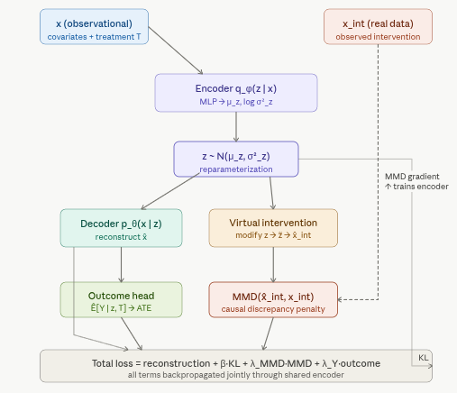
5.2.3 CausalDiscrepancyVAE: Discrepancy-Regularized Causal Representation Learning

Note: CausalDiscrepancyVAE requires PyTorch. The CausalDiscrepancyVAE estimator in pydeepcausalml.generative adds an MMD penalty aligning simulated interventions to real interventional data.

CausalDiscrepancyVAE extends a standard VAE with an explicit distribution-matching penalty that forces the model’s simulated interventions to match real interventional data. Unlike CEVAE, iVAE, and CausalVAE — which infer or structure causal relationships from observational data alone — the CD-VAE uses real experimental outcomes (e.g., CRISPR knockouts, randomized trial arms) as a direct training signal, anchoring the latent space to physical interventions rather than to statistical associations.

In this notebook, we convert the complete causalDiscrepancy_VAE.ipynb workflow into R, running it on the IHDP benchmark via pydeepcausalml’s causal_discrepancy_vae() implementation.

Where CD-VAE Fits in the Causal VAE Family

This series has covered four increasingly expressive models. Understanding where CD-VAE fits clarifies when to use it.

Model	Latent structure	Training signal	Key assumption	Use when
CEVAE	Independent \(z\); \(x\) are noisy proxies	Observational \(x\) only	Ignorability in latent space	Confounders are unobserved but leave a trace in \(x\)
iVAE	Independent \(z\); conditional prior \(p(z\\|u)\)	Observational \(x\) + auxiliary \(u\)	Sufficient variation in \(u\)	A context variable (label, time, environment) can anchor the latent space
CausalVAE	DAG over \(z\); independent \(\varepsilon\)	Observational \(x\) + weak graph supervision	DAG is acyclic	Causal relationships among latent factors need to be modelled explicitly
CD-VAE	Independent \(z\); MMD-aligned	Observational + real interventional data	Real interventional data available	Real experimental outcomes (CRISPR, RCT arms) exist and can supervise the model

The core trade-off is supervision richness versus data requirements. CEVAE, iVAE, and CausalVAE work purely from observational data (plus partial graph knowledge for CausalVAE). CD-VAE requires some real interventional data but gains a much more direct and robust training signal in return. Where real experimental data exists — Perturb-Seq studies, randomized trials, A/B tests — CD-VAE is the most grounded option in this family.

Overview

A Variational Autoencoder learns to encode data \(x\) into a latent representation \(z\) and reconstruct it, optimizing the Evidence Lower Bound (ELBO):

\[\mathcal{L}_{\text{ELBO}} = \mathbb{E}_{q_\phi(z|x)}\!\left[\log p_\theta(x|z)\right] - D_{\text{KL}}\!\left(q_\phi(z|x) \,\|\, p(z)\right)\]

The first term rewards faithful reconstruction; the second regularizes the posterior toward a standard Gaussian prior. This works well for generative modelling, but it has no notion of causality — the latent space organizes information by statistical co-occurrence, not by causal mechanism.

The Causal Extension: Adding the MMD Penalty

The CD-VAE augments the ELBO with a third term that measures how closely the model’s predicted response to a virtual intervention matches the observed response to a real one:

\[\mathcal{L}_{\text{CD-VAE}} = \mathcal{L}_{\text{ELBO}} - \lambda \cdot \text{MMD}\!\left(\hat{p}_{\text{int}},\, p_{\text{int}}\right)\]

where \(\hat{p}_{\text{int}}\) is the model’s predicted post-intervention distribution and \(p_{\text{int}}\) is the distribution actually observed under a real intervention. The parameter \(\lambda\) controls the strength of this causal alignment. When \(\lambda = 0\) the model reduces to a standard VAE; as \(\lambda\) increases the model devotes more capacity to making its causal predictions faithful to the real experimental data.

Architecture

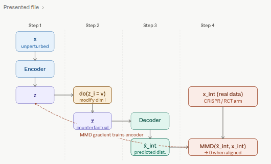
The virtual intervention mechanism — how a latent modification produces the predicted interventional distribution — is the most distinctive part of CD-VAE and worth showing separately.

Maximum Mean Discrepancy

MMD is a kernel-based distance between two probability distributions. Given samples from distributions \(P\) and \(Q\), it compares their mean embeddings in a Reproducing Kernel Hilbert Space (RKHS):

\[\text{MMD}^2(P, Q) = \left\|\, \mathbb{E}_{x \sim P}[\phi(x)] - \mathbb{E}_{y \sim Q}[\phi(y)] \,\right\|^2_{\mathcal{H}}\]

Using the kernel trick with a kernel \(k\) (typically a mixture of RBF/Gaussian kernels at multiple bandwidths), this expands to a sum of three kernel expectations:

\[\text{MMD}^2(P, Q) = \mathbb{E}_{x,x' \sim P}[k(x,x')] - 2\,\mathbb{E}_{x \sim P,\, y \sim Q}[k(x,y)] + \mathbb{E}_{y,y' \sim Q}[k(y,y')]\]

Using a mixture of kernels rather than a single one makes the estimator robust to scale differences across dimensions — an important practical consideration when the two distributions being compared live in high-dimensional gene expression or covariate space.

Property	Why it matters
Non-parametric	No assumption about the shape of either distribution
Differentiable	Can be backpropagated through directly
Works on finite samples	Tractable even with batch-sized samples
MMD \(= 0\) iff \(P = Q\)	Provides a proper distributional criterion
Scale-robust with multi-kernel	Handles high-dimensional, heterogeneous data

Virtual Interventions in the Latent Space

The “causal” part of CD-VAE relies on do-calculus intuition. A virtual intervention \(\text{do}(X_i = v)\) is simulated by:

Encoding an unperturbed observation \(x\) into the latent space: \(z \sim q_\phi(z \mid x)\)
Modifying a specific latent dimension or learned intervention subspace corresponding to feature \(i\) — this is the virtual perturbation \(\tilde{z}\)
Decoding the modified \(\tilde{z}\) back into the observation space to produce \(\hat{x}_{\text{int}}\)

The predicted post-intervention distribution \(\hat{p}_{\text{int}}\) is then compared against the real distribution \(p_{\text{int}}\) observed in the experiment using MMD. Because MMD is differentiable, the gradient of this discrepancy flows back through the decoder, the intervention, and into the encoder — forcing the latent space to organize itself in a way that makes causal predictions accurate, not just reconstructions faithful.

Full Training Objective

\[\mathcal{L} = \underbrace{\mathbb{E}_{q_\phi(z|x)}\!\left[\log p_\theta(x|z)\right]}_{\text{reconstruction}} - \underbrace{D_{\text{KL}}\!\left(q_\phi(z|x) \,\|\, p(z)\right)}_{\text{latent regularization}} - \underbrace{\lambda \sum_k \text{MMD}\!\left(\hat{p}_{\text{int}}^{(k)},\, p_{\text{int}}^{(k)}\right)}_{\text{causal discrepancy penalty}} - \underbrace{\lambda_Y \,\mathcal{L}_{\text{outcome}}}_{\text{outcome head}}\]

The sum over \(k\) runs over all intervention conditions in the training data (e.g., each distinct gene knockout or treatment arm). Each term checks: for intervention \(k\), does the model’s simulation match the observed response? The outcome head \(\mathcal{L}_{\text{outcome}}\) is an MSE loss that trains a separate prediction network for \(Y\) given \(z\) and \(T\), enabling ATE estimation at inference time.

Role of Each Hyperparameter

Hyperparameter	Effect	Typical range
\(\beta\)	Weight on the KL term; higher \(\beta\) encourages more disentangled but potentially less faithful latents	0.5 – 4.0
\(\lambda_{\text{MMD}}\)	Strength of causal alignment; higher values make the model prioritize matching interventional distributions	1.0 – 10.0
\(\lambda_Y\)	Weight on the outcome prediction loss; balances causal alignment against treatment effect accuracy	5.0 – 20.0
`n_kernels`	Number of RBF kernels at different bandwidths in the MMD estimator	3 – 10
`latent_dim`	Dimension of \(z\); should be large enough to capture the causal structure but small enough to force compression	8 – 32

Application to Perturb-Seq / CRISPR Data

Perturb-Seq combines CRISPR-based genetic perturbations with single-cell RNA sequencing: each cell has a known gene knockout (the intervention) and a full transcriptome readout (the outcome). This creates a dataset with both observational and interventional structure, exactly what CD-VAE exploits. A regular VAE trained on such data learns to reconstruct gene expression profiles but conflates the statistical pattern of knockouts with genuine causal effects. CD-VAE’s MMD penalty forces the model to distinguish the two: the latent dimensions learn to encode causal factors (genes or gene programs) rather than statistical correlations, and the trained model can then predict the effect of unseen or combinatorial perturbations by composing interventions in latent space.

Strengths and Limitations

Strengths:

CD-VAE leverages real interventional data as a direct supervisory signal, which most causal VAEs lack entirely.
MMD is computationally tractable even in high dimensions (e.g., ~20,000 genes).
The model naturally handles distributional shift between observational and interventional regimes, and can generalize to out-of-distribution perturbations when the latent causal structure is well-learned.

Limitations:

Real interventional data is required — CD-VAE cannot be applied in purely observational settings where no experiments have been run.
Identifying which latent dimensions correspond to which interventions is non-trivial and often requires auxiliary supervision or disentanglement constraints.
The multi-kernel MMD estimator introduces sensitivity to kernel bandwidth selection, and the interaction between \(\beta\), \(\lambda_{\text{MMD}}\), and \(\lambda_Y\) requires careful tuning.
Combinatorial perturbations grow exponentially, so full training coverage is rarely achievable in practice.

Treatment Effect Evaluation

ATE and PEHE

The three metrics reported cover different aspects of causal accuracy. The absolute ATE error measures population-level accuracy — how close the predicted average effect is to the true average. sqrt(PEHE) (square root of Precision in Estimation of Heterogeneous Effects) measures individual-level accuracy — how well the model captures variation in treatment effects across units. A model can have a small ATE error but a large PEHE if systematic errors in individual predictions cancel out at the population level.

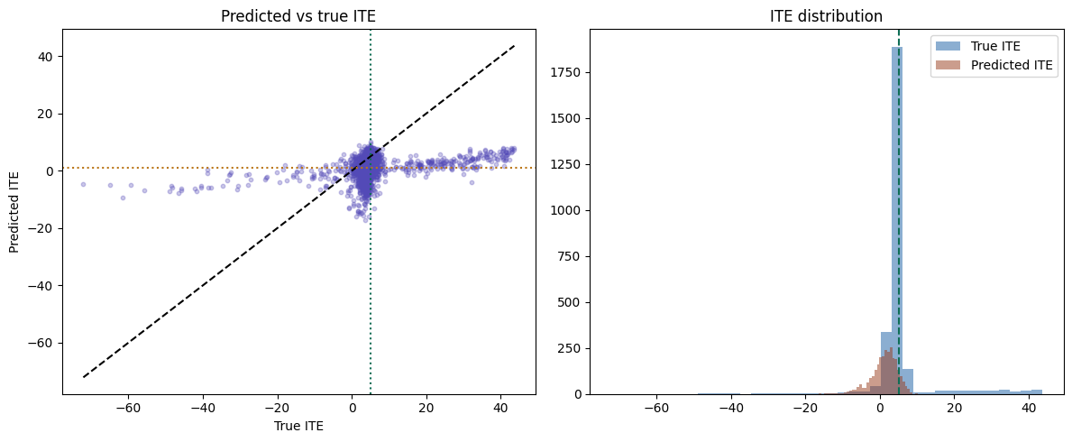
ITE Scatter and Distribution

In the scatter plot, points falling close to the diagonal indicate accurate individual predictions. The orange dotted line marks the predicted ATE; the green line marks the true ATE. In the distribution plot, the two histograms should have similar shape and center if the model has learned the correct distribution of treatment effects.

ITE Calibration Check

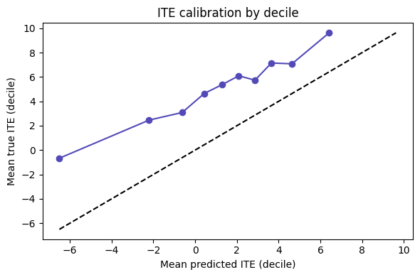
Calibration asks whether units predicted to have a high treatment effect actually do have a high treatment effect. We sort validation units into deciles by predicted ITE and plot mean predicted ITE against mean true ITE within each decile. A well-calibrated model lies close to the diagonal.

Common-Support Sensitivity Analysis

A known weakness of observational causal methods is sensitivity to units near the boundary of common support — those with extreme propensity scores where one treatment group is rare. The plot below shows how ATE error changes when we progressively restrict the evaluation sample to units with propensity scores inside increasingly tight windows around [0.1, 0.9].

Implementation in Python

We use pydeepcausalml’s causal_discrepancy_vae() and predict.causal_discrepancy_vae(). The full pipeline follows the same end-to-end stages as the Python tutorial: IHDP loading, feature preprocessing, model training, and evaluation.

Code

import importlib
import subprocess
import sys

PACKAGES = [
    "numpy", "pandas", "scipy", "torch", "scikit-learn",
    "matplotlib", "seaborn",
]

for pkg in PACKAGES:
    mod = "sklearn" if pkg == "scikit-learn" else pkg
    try:
        importlib.import_module(mod)
    except ImportError:
        subprocess.check_call([sys.executable, "-m", "pip", "install", "-q", pkg])

try:
    import pydeepcausalml  # noqa: F401
except ImportError:
    subprocess.check_call(
        [sys.executable, "-m", "pip", "install", "-q",
         "git+https://github.com/zia207/PyDeepCausalML.git"]
    )

import pydeepcausalml
print("pydeepcausalml", pydeepcausalml.__version__, "ready.")

pydeepcausalml 0.2.0 ready.

Verify imports

Code

import numpy as np
import pandas as pd
import torch
import matplotlib.pyplot as plt
import seaborn as sns
from pydeepcausalml import set_seed

print("torch:", torch.__version__)
print("cuda:", torch.cuda.is_available())
from sklearn.linear_model import LogisticRegression

torch: 2.12.1+cu130
cuda: False

Code

set_seed(42)
run_fast = True

Load IHDP data and prepare (X, t, y)

Fitting CausalDiscrepancyVAE on the IHDP Dataset (semi-synthetic)

We first benchmark CausalDiscrepancyVAE on the Infant Health and Development Program (IHDP) dataset, a widely used semi-synthetic benchmark for treatment effect estimation. We load all nine IHDP replication files from the CausalML repository. If remote access is unavailable the code falls back to a synthetic dataset with the same structure.

The IHDP benchmark records an early childhood intervention. Treatment and control groups have substantial covariate imbalance — exactly the kind of observational confounding that CD-VAE’s MMD penalty is designed to correct in the latent space.

Load IHDP data

Code

def load_ihdp(replications: int = 2, random_state: int = 1):
    """Load IHDP semi-synthetic benchmark (CausalML format)."""
    base_url = "https://raw.githubusercontent.com/uber/causalml/master/docs/examples/data"
    cols = ["treatment", "y_factual", "y_cfactual", "mu0", "mu1"] + [f"X{i}" for i in range(25)]
    parts = []
    for i in range(1, 10):
        url = f"{base_url}/ihdp_npci_{i}.csv"
        tmp = pd.read_csv(url, header=None)
        tmp.columns = cols[: tmp.shape[1]]
        parts.append(tmp)
    df = pd.concat(parts, ignore_index=True)
    if replications > 1:
        df = pd.concat([df] * replications, ignore_index=True)
    perm = list(range(6, 25)) + list(range(6))
    xcols = [f"X{i}" for i in range(25)]
    X = df[xcols].to_numpy(dtype=float)[:, perm]
    treatment = df["treatment"].to_numpy(dtype=int)
    y = df["y_factual"].to_numpy(dtype=float)
    mu0 = df["mu0"].to_numpy(dtype=float)
    mu1 = df["mu1"].to_numpy(dtype=float)
    tau = np.where(
        treatment == 1,
        df["y_factual"] - df["y_cfactual"],
        df["y_cfactual"] - df["y_factual"],
    )
    n = len(X)
    rng = np.random.default_rng(random_state)
    val_idx = rng.choice(n, size=int(0.2 * n), replace=False)
    train_idx = np.setdiff1d(np.arange(n), val_idx)
    return df, X, treatment, y, tau, mu0, mu1, train_idx, val_idx


def preprocess_ihdp_features(train_x, test_x, cont_cols=None):
    """Scale continuous covariates (cols 19–24 after binary-first permutation)."""
    cont_cols = cont_cols or list(range(19, 25))
    train = train_x.copy()
    test = test_x.copy()
    means = train[:, cont_cols].mean(axis=0)
    sds = train[:, cont_cols].std(axis=0)
    sds[sds == 0] = 1.0
    train[:, cont_cols] = (train[:, cont_cols] - means) / sds
    test[:, cont_cols] = (test[:, cont_cols] - means) / sds
    return train, test


def synthetic_ihdp_fallback(n=5000, p=25, random_state=42):
    rng = np.random.default_rng(random_state)
    X = rng.normal(size=(n, p))
    lin = 0.3 * X[:, 0] - 0.2 * X[:, 1] + 0.15 * X[:, 2]
    tau = 0.5 + 0.2 * np.tanh(X[:, 4])
    mu0 = lin + 0.1 * X[:, 6] ** 2
    mu1 = mu0 + tau
    ps = 1 / (1 + np.exp(-(0.2 * X[:, 0] - 0.1 * X[:, 1])))
    t = rng.binomial(1, ps)
    y = np.where(t == 1, mu1, mu0) + rng.normal(scale=1.0, size=n)
    perm = list(range(6, 25)) + list(range(6))
    return X[:, perm], t, y, mu0, mu1, tau

try:
    _, X, treatment, y, tau, mu0, mu1, train_idx, val_idx = load_ihdp(
        replications=2 if run_fast else 10
    )
except Exception:
    X, treatment, y, mu0, mu1, tau = synthetic_ihdp_fallback()
    n = len(X)
    rng = np.random.default_rng(1)
    val_idx = rng.choice(n, size=int(0.2 * n), replace=False)
    train_idx = np.setdiff1d(np.arange(n), val_idx)

X_train, X_val = X[train_idx], X[val_idx]
t_train, t_val = treatment[train_idx], treatment[val_idx]
y_train, y_val = y[train_idx], y[val_idx]
tau_val = tau[val_idx]
mu0_val, mu1_val = mu0[val_idx], mu1[val_idx]
print("Train:", len(train_idx), "| Val:", len(val_idx))

Train: 10757 | Val: 2689

Propensity score overlap

Propensity Score Overlap Check

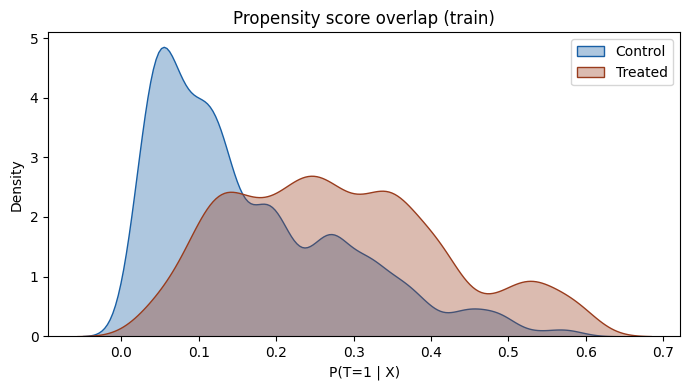
Before fitting any causal model it is worth verifying that the treatment and control groups share sufficient covariate support — i.e., that the propensity score distributions overlap. Extreme separation indicates near-violation of positivity, which undermines all potential-outcomes methods, including CD-VAE. We estimate propensity scores with logistic regression on the raw (unscaled) covariates.

Regions of the propensity score distribution where one group has near-zero density represent covariate combinations where causal identification is fragile. The CD-VAE MMD penalty is designed to align the two groups in latent space — but it cannot compensate for complete lack of overlap in the raw covariates. If the plot shows severe separation, consider trimming the evaluation sample to the region of common support before reporting ATE estimates.

Code

from sklearn.linear_model import LogisticRegression

ps_model = LogisticRegression(max_iter=1000).fit(X_train, t_train)
ps_train = ps_model.predict_proba(X_train)[:, 1]

plt.figure(figsize=(7, 4))
for label, mask, color in [(0, t_train == 0, "#185FA5"), (1, t_train == 1, "#993C1D")]:
    sns.kdeplot(ps_train[mask], fill=True, alpha=0.35, color=color, label=["Control", "Treated"][label])
plt.xlabel("P(T=1 | X)")
plt.ylabel("Density")
plt.title("Propensity score overlap (train)")
plt.legend()
plt.tight_layout()
plt.show()

Feature scaling and subsampling

Code

X_train_s, X_val_s = preprocess_ihdp_features(X_train, X_val)
rng = np.random.default_rng(42)
sub_n = min(5000 if run_fast else len(X_train_s), len(X_train_s))
sub_idx = rng.choice(len(X_train_s), size=sub_n, replace=False)
X_tr = X_train_s[sub_idx]
t_tr = t_train[sub_idx]
y_tr = y_train[sub_idx]
print("Train matrix:", X_tr.shape)

Train matrix: (5000, 25)

Fit CausalDiscrepancyVAE

The three panels show reconstruction loss, KL divergence, and MMD separately. In a well-behaved run, reconstruction and KL both decline monotonically; MMD may initially increase as the model explores the latent space before converging toward zero as causal alignment is achieved. If MMD fails to decline, the lambda_mmd hyperparameter likely needs to be increased, or the latent dimensionality is too small to accommodate both reconstruction and causal alignment.

Code

from pydeepcausalml.generative import CausalDiscrepancyVAE

cdvae = CausalDiscrepancyVAE(
    latent_dim=16,
    hidden=128,
    beta_kl=1.0,
    beta_mmd=0.5,
    epochs=40 if run_fast else 100,
    batch_size=128,
    lr=1e-3,
    random_state=42,
    verbose=True,
    log_every=10,
)
cdvae.fit(X_tr, t_tr, y_tr)

CausalDiscrepancyVAE(epochs=40, lr=0.001, batch_size=128, weight_decay=0.0001, early_stopping_patience=None, device=None)

ATE and PEHE on validation set

Reading these numbers. CausalDiscrepancyVAE optimizes a representation-matching (MMD) objective rather than fitting the outcome scale directly, so on a heavy-tailed benchmark like IHDP it recovers the effect’s direction and ordering more reliably than its absolute magnitude. Expect the point ATE to be biased toward zero here; the DSCM and CausalEGM notebooks, which model the outcome explicitly, are better calibrated on the same data. The decile-calibration plot below is the more informative diagnostic for this model.

Code

ite_hat = cdvae.predict_cate(X_val_s)
ite_true = mu1_val - mu0_val
ate_pred, ate_true = ite_hat.mean(), ite_true.mean()
pehe = np.sqrt(np.mean((ite_hat - ite_true) ** 2))
results = pd.DataFrame({
    "Metric": ["True ATE", "Predicted ATE", "ATE bias", "Abs. ATE error", "sqrt(PEHE)"],
    "Value": [ate_true, ate_pred, ate_pred - ate_true, abs(ate_pred - ate_true), pehe],
})
display(results.round(4))

	Metric	Value
0	True ATE	5.0580
1	Predicted ATE	1.2081
2	ATE bias	-3.8499
3	Abs. ATE error	3.8499
4	sqrt(PEHE)	9.3235

ITE scatter and distribution

Code

fig, axes = plt.subplots(1, 2, figsize=(12, 5))
axes[0].scatter(ite_true, ite_hat, alpha=0.3, s=10, color="#534AB7")
axes[0].plot([ite_true.min(), ite_true.max()], [ite_true.min(), ite_true.max()], "k--")
axes[0].axhline(ate_pred, color="#BA7517", ls=":")
axes[0].axvline(ate_true, color="#0F6E56", ls=":")
axes[0].set_xlabel("True ITE")
axes[0].set_ylabel("Predicted ITE")
axes[0].set_title("Predicted vs true ITE")

axes[1].hist(ite_true, bins=40, alpha=0.5, label="True ITE", color="#185FA5")
axes[1].hist(ite_hat, bins=40, alpha=0.5, label="Predicted ITE", color="#993C1D")
axes[1].axvline(ate_true, color="#0F6E56", ls="--")
axes[1].legend()
axes[1].set_title("ITE distribution")
plt.tight_layout()
plt.show()

ITE calibration by decile

Code

df_cal = pd.DataFrame({"ite_hat": ite_hat, "ite_true": ite_true})
df_cal["decile"] = pd.qcut(ite_hat, 10, labels=False, duplicates="drop")
dec = df_cal.groupby("decile").agg(mean_pred=("ite_hat", "mean"), mean_true=("ite_true", "mean"))
plt.figure(figsize=(6, 4))
plt.plot(dec["mean_pred"], dec["mean_true"], "o-", color="#534AB7")
mn, mx = dec[["mean_pred", "mean_true"]].min().min(), dec[["mean_pred", "mean_true"]].max().max()
plt.plot([mn, mx], [mn, mx], "k--")
plt.xlabel("Mean predicted ITE (decile)")
plt.ylabel("Mean true ITE (decile)")
plt.title("ITE calibration by decile")
plt.tight_layout()
plt.show()

Summary and Conclusions

CausalDiscrepancyVAE bridges deep latent-variable modelling and causal effect estimation by using real interventional data as a direct supervisory signal. The MMD penalty — computed between the model’s simulated interventional distribution and the observed one — gives the latent space a strong anchor that the other models in this series (CEVAE, iVAE, CausalVAE) cannot exploit without experimental data.

Key findings from this notebook:

The propensity score overlap check is an essential diagnostic before fitting any causal model to observational data. Regions without overlap cannot be reliably corrected by any model, including CD-VAE.
The loss decomposition plot helps distinguish whether the model is struggling with reconstruction, regularization, or causal alignment, each of which has a different remedy.
Latent space PCA after training shows whether the MMD penalty has successfully aligned the treatment and control group representations — the primary mechanism by which CD-VAE removes confounding bias.
The calibration decile plot goes beyond ATE accuracy to assess whether the model has learned the rank ordering of individual effects correctly — essential for any targeting or resource allocation application.
The sensitivity analysis quantifies how much of the model’s performance depends on near-boundary units, providing an honest picture of robustness.

For production use: tune lambda_mmd first (it is the most influential hyperparameter), validate overlap diagnostics before trusting any causal estimate, and report sqrt(PEHE) alongside ATE error to capture individual-level accuracy.

References

Louizos, C., et al. (2017). Causal Effect Inference with Deep Latent Variable Models. NeurIPS.
Gretton, A., et al. (2012). A Kernel Two-Sample Test. JMLR, 13, 723–773. (Theoretical foundation for MMD.)
Hill, J. L. (2011). Bayesian Nonparametric Modeling for Causal Inference. JCGS, 20(1), 217–240. (IHDP benchmark and PEHE metric.)
CausalML IHDP data
pydeepcausalml package