Python Banner

5.1.4 GANITE: Generative Adversarial Network for Inference of Treatment Effects

GANITE (Yoon, Jordon, and van der Schaar, 2018) estimates individual treatment effects (ITE) by recasting the counterfactual inference problem as a generative modeling task. The core challenge it addresses is fundamental to causal inference: for any individual, only the outcome under the treatment they actually received is ever observed, while the outcome under the alternative treatment remains counterfactual and unknowable. Rather than imputing a single point estimate for this missing outcome, GANITE uses a Generative Adversarial Network to learn the full distribution of potential outcomes — capturing uncertainty while remaining grounded in the observed data distribution.

Overview

GANITE (Yoon, Jordon, and van der Schaar, 2018) estimates individual treatment effects (ITE) by recasting counterfactual inference as a generative modeling task. The core challenge it addresses is fundamental to causal inference: for any individual, only the outcome under the treatment they actually received is observable, while the outcome under the alternative treatment remains counterfactual and unknowable. Rather than imputing a single point estimate for this missing outcome, GANITE uses a two-block GAN to learn the full distribution of potential outcomes — capturing epistemic uncertainty while remaining grounded in the observed data distribution.

In the potential outcomes framework, for each individual i we observe covariates \(X_i\), treatment \(T_i \in \{0, 1\}\), and factual outcome \(Y_i^F = Y_i(T_i)\). The counterfactual outcome \(Y_i^{CF} = Y_i(1 - T_i)\) is never observed. The individual treatment effect is therefore:

\[\tau_i = Y_i(1) - Y_i(0)\]

Standard regression models impute a single value for the missing \(Y_i^{CF}\). GANITE instead learns a conditional generative model \(p(Y(0), Y(1) \mid X)\), from which both potential outcomes and their uncertainty can be sampled.

The two-block architecture

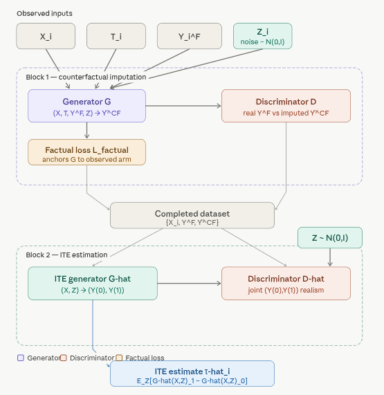
GANITE cleanly separates two sub-problems: imputing missing counterfactuals (Block 1) and estimating treatment effects from the completed data (Block 2). The diagram below shows GANITE’s overall two-block pipeline from inputs through to the ITE estimate.

Block 1 — the counterfactual generator. The generator \(G\) takes the observed tuple \((X_i, T_i, Y_i^F)\) together with a noise vector \(Z_i \sim \mathcal{N}(0, I)\) and outputs an imputed counterfactual \(\tilde{Y}_i^{CF}\). A discriminator \(D\) is trained to distinguish real factual outcomes from generator-imputed counterfactuals, forcing \(G\) to produce counterfactuals that are indistinguishable in distribution from real outcomes. A factual reconstruction term \(\mathcal{L}_\text{factual}\) anchors the generator to the observed arm, preventing it from producing well-distributed but causally meaningless imputations.

Block 2 — the ITE generator. Once Block 1 has produced imputed counterfactuals for every training individual, a second generator \(\hat{G}\) is trained on the now-complete dataset \(\{X_i, \tilde{Y}_i^{CF}, Y_i^F\}\). Unlike \(G\), it takes only covariates and noise as input — treatment and factual outcome are no longer needed because the missing data problem has been resolved. A second discriminator \(\hat{D}\) distinguishes \(\hat{G}\)’s joint outcome pairs from the Block 1 pairs, ensuring the joint distribution of \((Y(0), Y(1))\) is respected rather than just the marginals independently. The final ITE estimate averages over multiple noise draws:

\[\hat{\tau}_i = \mathbb{E}_Z[\hat{G}(X_i, Z)_1 - \hat{G}(X_i, Z)_0]\]

Combined training objective:

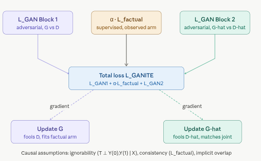
\[\mathcal{L} = \mathcal{L}_\text{GAN}^\text{Block 1} + \alpha \cdot \mathcal{L}_\text{factual} + \mathcal{L}_\text{GAN}^\text{Block 2}\]

The shows how the three loss terms combine and the direction of gradient flow during training.

Causal assumptions encoded

GANITE encodes three standard causal assumptions through its architecture. It assumes ignorability — that \(T \perp (Y(0), Y(1)) \mid X\), meaning all confounding is captured in the observed covariates. It enforces consistency through the factual reconstruction loss, which requires \(\hat{Y}_i(T_i) \approx Y_i^F\). It does not explicitly enforce overlap, but the adversarial training implicitly pressures the generator to produce plausible outcomes across both treatment arms for all covariate values.

Uncertainty quantification

One of GANITE’s most distinctive properties relative to deterministic estimators like TARNet or DragonNet is its native uncertainty quantification. Because both generators are stochastic, repeated forward passes through \(\hat{G}\) yield a distribution over ITE estimates:

\[\{\hat{\tau}_i^{(k)}\}_{k=1}^K = \{\hat{G}(X_i, Z^{(k)})_1 - \hat{G}(X_i, Z^{(k)})_0\}_{k=1}^K\]

This distribution reflects genuine epistemic uncertainty about the unobservable counterfactual — not merely variance from model fitting. Point-estimate models cannot provide this without additional machinery such as bootstrapping or conformal prediction. GANITE’s generative approach captures it directly in the model’s output distribution.

Relationship to Other Methods

Method Generative Uncertainty Latent Confounders Architecture
TARNet No No No Shared encoder + two heads
CFRNet No No No TARNet + MMD balancing
DragonNet No No No TARNet + propensity head
GANITE Yes (GAN) Yes No Two-block GAN

GANITE is a generative model that captures uncertainty while operating in observed covariate space like TARNet, rather than learning a latent confounder structure.

Assumptions and Limitations

Assumptions: - Strong ignorability holds in observed covariate space X - The GAN generator is expressive enough to capture the true distribution of potential outcomes - Sufficient sample size to train two coupled adversarial networks stably

Limitations: - GAN training is notoriously unstable — mode collapse, vanishing gradients, and sensitivity to hyperparameters are all practical concerns - The two-block training is sequential, meaning errors in Block 1 (counterfactual imputation) propagate into Block 2 (ITE estimation) with no mechanism to correct them - Evaluation is difficult because counterfactuals are never observed; standard loss functions cannot directly measure counterfactual accuracy on real data - Computationally expensive relative to simpler regression-based ITE estimators

Implementation in Python

We implement GANITE with PyDeepCausalML and compare it to meta-learners (S, T, X, R) on the IHDP semi-synthetic dataset and a synthetic dataset with hidden confounding.

Check and Install Required Python Packages

The following packages are used in this notebook. Install any missing packages with the cell below:

numpy, pandas, scipy, torch, scikit-learn, matplotlib, seaborn, causaldata, pydeepcausalml

Code
import importlib
import subprocess
import sys
from pathlib import Path

PACKAGES = [
    "numpy", "pandas", "scipy", "torch", "scikit-learn",
    "matplotlib", "seaborn", "causaldata",
]

for pkg in PACKAGES:
    mod = "sklearn" if pkg == "scikit-learn" else pkg
    try:
        importlib.import_module(mod)
    except ImportError:
        subprocess.check_call([sys.executable, "-m", "pip", "install", "-q", pkg])

try:
    import pydeepcausalml  # noqa: F401
except ImportError:
    repo_root = Path("..").resolve()
    subprocess.check_call([sys.executable, "-m", "pip", "install", "-q", "-e", str(repo_root)])

print("Packages ready.")

Verify imports

Code
import numpy as np
import pandas as pd
import torch
import matplotlib.pyplot as plt
import seaborn as sns
from pydeepcausalml import set_seed

print("torch:", torch.__version__)
print("cuda:", torch.cuda.is_available())
Code
from pathlib import Path
import os
import numpy as np
import pandas as pd
from sklearn.ensemble import RandomForestRegressor
from sklearn.linear_model import ElasticNet, LogisticRegression, LinearRegression
from sklearn.model_selection import KFold


def load_nsw_mixtape() -> pd.DataFrame:
    """Load NSW (Lalonde) mixtape data (same variables as causaldata::nsw_mixtape)."""
    try:
        import causaldata.nsw_mixtape.data as nsw_data
        dta = Path(nsw_data.__file__).parent / "nsw_mixtape.dta"
        return pd.read_stata(dta)
    except Exception:
        pass
    url = (
        "https://raw.githubusercontent.com/NickCH-K/causaldata/master/"
        "data-raw/nsw_mixtape.dta"
    )
    return pd.read_stata(url)


def propensity_elastic_net(X: np.ndarray, treatment: np.ndarray) -> np.ndarray:
    model = LogisticRegression(
        penalty="elasticnet", solver="saga", l1_ratio=0.5, max_iter=2000
    )
    model.fit(X, treatment)
    return model.predict_proba(X)[:, 1]


class SLearner:
    def __init__(self, learner: str = "ranger"):
        self.learner = learner

    def fit(self, X, t, y):
        Xt = np.column_stack([X, t])
        if self.learner == "lm":
            self.model_ = LinearRegression().fit(Xt, y)
        else:
            self.model_ = RandomForestRegressor(
                n_estimators=100, random_state=42, n_jobs=-1
            ).fit(Xt, y)
        return self

    def predict(self, X):
        y0 = self.model_.predict(np.column_stack([X, np.zeros(len(X))]))
        y1 = self.model_.predict(np.column_stack([X, np.ones(len(X))]))
        return y1 - y0


class TLearner:
    def __init__(self, learner: str = "ranger"):
        self.learner = learner

    def fit(self, X, t, y):
        t = t.astype(int)
        if self.learner == "lm":
            self.m0_ = LinearRegression().fit(X[t == 0], y[t == 0])
            self.m1_ = LinearRegression().fit(X[t == 1], y[t == 1])
        else:
            self.m0_ = RandomForestRegressor(
                n_estimators=100, random_state=42, n_jobs=-1
            ).fit(X[t == 0], y[t == 0])
            self.m1_ = RandomForestRegressor(
                n_estimators=100, random_state=42, n_jobs=-1
            ).fit(X[t == 1], y[t == 1])
        return self

    def predict(self, X):
        return self.m1_.predict(X) - self.m0_.predict(X)


class XLearner:
    def __init__(self, learner: str = "ranger"):
        self.learner = learner

    def _reg(self):
        if self.learner == "lm":
            return LinearRegression()
        return RandomForestRegressor(n_estimators=100, random_state=42, n_jobs=-1)

    def fit(self, X, t, y, p=None):
        t = t.astype(int)
        self.propensity_model_ = LogisticRegression(
            penalty="elasticnet", solver="saga", l1_ratio=0.5, max_iter=2000
        ).fit(X, t)
        m0, m1 = self._reg(), self._reg()
        m0.fit(X[t == 0], y[t == 0])
        m1.fit(X[t == 1], y[t == 1])
        d1 = y[t == 1] - m0.predict(X[t == 1])
        d0 = m1.predict(X[t == 0]) - y[t == 0]
        tau1 = self._reg().fit(X[t == 1], d1)
        tau0 = self._reg().fit(X[t == 0], d0)
        self.tau0_, self.tau1_ = tau0, tau1
        return self

    def predict(self, X):
        p = self.propensity_model_.predict_proba(X)[:, 1]
        return p * self.tau0_.predict(X) + (1 - p) * self.tau1_.predict(X)


class RLearner:
    def __init__(self, learner: str = "ranger", n_fold: int = 3):
        self.learner = learner
        self.n_fold = n_fold

    def _reg(self):
        if self.learner == "lm":
            return LinearRegression()
        return RandomForestRegressor(n_estimators=100, random_state=42, n_jobs=-1)

    def fit(self, X, t, y, p=None):
        t = t.astype(int).astype(float)
        p = propensity_elastic_net(X, t) if p is None else p
        e = t - p
        m = self._reg()
        kf = KFold(n_splits=self.n_fold, shuffle=True, random_state=42)
        y_hat = np.zeros_like(y, dtype=float)
        for tr, va in kf.split(X):
            m.fit(X[tr], y[tr])
            y_hat[va] = m.predict(X[va])
        resid = y - y_hat
        tau = self._reg()
        tau.fit(X, resid / (e + 1e-6), sample_weight=e**2)
        self.tau_ = tau
        return self

    def predict(self, X):
        return self.tau_.predict(X)


def get_cumgain(df_preds, outcome_col="y", treatment_col="w", treatment_effect_col="tau", normalize=True):
    """Cumulative gain curve (CausalML-style AUUC helper)."""
    y = df_preds[outcome_col].to_numpy()
    w = df_preds[treatment_col].to_numpy()
    tau = df_preds[treatment_effect_col].to_numpy()
    model_cols = [c for c in df_preds.columns if c not in {outcome_col, treatment_col, treatment_effect_col}]
    n = len(df_preds)
    out = {}
    for col in model_cols:
        scores = df_preds[col].to_numpy()
        order = np.argsort(-scores)
        cum = []
        treated_so_far = control_so_far = 0.0
        for i, idx in enumerate(order, start=1):
            if w[idx] == 1:
                treated_so_far += y[idx]
            else:
                control_so_far += y[idx]
            lift = treated_so_far / max((w[order[:i]] == 1).sum(), 1) - control_so_far / max(
                (w[order[:i]] == 0).sum(), 1
            )
            cum.append(lift)
        curve = np.array(cum)
        if normalize and curve[-1] != 0:
            curve = curve / np.abs(curve[-1])
        out[col] = curve
    out[treatment_effect_col] = out.get(treatment_effect_col, out[model_cols[0]])
    return pd.DataFrame(out)


def plot_gain(df_preds, outcome_col="y", treatment_col="w", treatment_effect_col="tau", model_cols=None, main="", normalize=True):
    import matplotlib.pyplot as plt

    gain = get_cumgain(df_preds, outcome_col, treatment_col, treatment_effect_col, normalize)
    model_cols = model_cols or [c for c in gain.columns]
    plt.figure(figsize=(8, 5))
    for col in model_cols:
        if col in gain.columns:
            plt.plot(gain[col].values, label=col)
    plt.xlabel("Population fraction targeted")
    plt.ylabel("Cumulative gain" + (" (normalized)" if normalize else ""))
    plt.title(main)
    plt.legend()
    plt.tight_layout()
    plt.show()


def load_ihdp(replications: int = 2, random_state: int = 1):
    base_url = "https://raw.githubusercontent.com/uber/causalml/master/docs/examples/data"
    cols = ["treatment", "y_factual", "y_cfactual", "mu0", "mu1"] + [f"X{i}" for i in range(25)]
    parts = []
    for i in range(1, 10):
        url = f"{base_url}/ihdp_npci_{i}.csv"
        tmp = pd.read_csv(url, header=None)
        tmp.columns = cols[: tmp.shape[1]]
        parts.append(tmp)
    df = pd.concat(parts, ignore_index=True)
    if replications > 1:
        df = pd.concat([df] * replications, ignore_index=True)
    binfeats = [f"X{i}" for i in range(6, 25)]
    contfeats = [f"X{i}" for i in range(6)]
    xcols = binfeats + contfeats
    X = df[xcols].to_numpy(dtype=float)
    treatment = df["treatment"].to_numpy(dtype=int)
    y = df["y_factual"].to_numpy(dtype=float)
    tau = np.where(
        treatment == 1,
        df["y_factual"] - df["y_cfactual"],
        df["y_cfactual"] - df["y_factual"],
    )
    n = len(X)
    rng = np.random.default_rng(random_state)
    val_idx = rng.choice(n, size=int(0.2 * n), replace=False)
    train_idx = np.setdiff1d(np.arange(n), val_idx)
    return df, X, treatment, y, tau, train_idx, val_idx


def simulate_hidden_confounder(n=2000, p=5, sigma=1.0, adj=0, random_state=42):
    """Synthetic DGP with latent confounder (CausalML-style benchmark)."""
    rng = np.random.default_rng(random_state)
    z = rng.normal(size=n)
    X = np.column_stack([z + rng.normal(scale=sigma, size=n) for _ in range(p)])
    e = 1 / (1 + np.exp(-(adj + 0.5 * z)))
    w = rng.binomial(1, e)
    b = 2 * z + rng.normal(scale=sigma, size=n)
    tau = 0.5 + 0.3 * z
    y = b + w * tau + rng.normal(scale=sigma, size=n)
    return {"X": X, "y": y, "w": w, "tau": tau, "b": b, "e": e}


def result_table(df_preds, tau_true):
    model_cols = [c for c in ["S", "T", "X", "R", "GANITE", "CEVAE"] if c in df_preds.columns]
    methods = model_cols + ["actual"]
    ate = [df_preds[m].mean() for m in model_cols] + [float(tau_true.mean())]
    mae = [float(np.mean(np.abs(df_preds[m] - tau_true))) for m in model_cols] + [np.nan]
    gain = get_cumgain(df_preds)
    auuc = [float(gain[m].mean()) if m in gain.columns else np.nan for m in model_cols]
    auuc.append(float(gain["tau"].mean()) if "tau" in gain.columns else np.nan)
    return pd.DataFrame({"Method": methods, "ATE": ate, "MAE": mae, "AUUC": auuc})


def synthetic_summary(preds, tau_ref, actual_ate):
    rows = []
    for name, p in preds.items():
        rows.append({
            "Method": name,
            "ATE": p.mean(),
            "MSE": np.mean((p - tau_ref) ** 2),
            "AbsPctErrorATE": abs(p.mean() / actual_ate - 1) if actual_ate != 0 else np.nan,
        })
    rows.append({"Method": "Actuals", "ATE": actual_ate, "MSE": np.nan, "AbsPctErrorATE": np.nan})
    return pd.DataFrame(rows)

import os
from pydeepcausalml.effect import GANITE

RUN_FAST = os.getenv("PYDEEPCAUSALML_FAST_RENDER", "true").lower() == "true"
set_seed(42)

Fit GANITE on the IHDP dataset

Code
df, X, treatment, y, tau, train_idx, val_idx = load_ihdp(
    replications=2 if RUN_FAST else 10, random_state=1
)
X_train, X_val = X[train_idx], X[val_idx]
treatment_train, treatment_val = treatment[train_idx], treatment[val_idx]
y_train, y_val = y[train_idx], y[val_idx]
tau_train, tau_val = tau[train_idx], tau[val_idx]
print("Train size:", len(train_idx), "| Val size:", len(val_idx))

Fit GANITE model

Code
gn = GANITE(
    h_dim=25 if RUN_FAST else 50,
    epochs=100 if RUN_FAST else 500,
    batch_size=128 if RUN_FAST else 64,
    lr=1e-4,
    random_state=42,
    verbose=not RUN_FAST,
    log_every=20,
).fit(X_train, treatment_train, y_train)

ite_train_ganite = gn.predict_cate(X_train)
ite_val_ganite = gn.predict_cate(X_val)
print("GANITE — ATE (train):", round(ite_train_ganite.mean(), 4),
      "| ATE (val):", round(ite_val_ganite.mean(), 4))

Fit Meta-learners

Code
p_train = propensity_elastic_net(X_train, treatment_train)
n_fold_meta = 3 if RUN_FAST else 5
sl = SLearner("ranger").fit(X_train, treatment_train, y_train)
tl = TLearner("ranger").fit(X_train, treatment_train, y_train)
xl = XLearner("ranger").fit(X_train, treatment_train, y_train, p=p_train)
rl = RLearner("ranger", n_fold=n_fold_meta).fit(X_train, treatment_train, y_train, p=p_train)

Model results comparison — Training

Code
df_preds_train = pd.DataFrame({
    "S": sl.predict(X_train), "T": tl.predict(X_train),
    "X": xl.predict(X_train), "R": rl.predict(X_train),
    "GANITE": ite_train_ganite, "tau": tau_train,
    "w": treatment_train, "y": y_train,
})

display(result_table(df_preds_train, tau_train).round(4))
plot_gain(df_preds_train, main="Cumulative gain (Training)")

Validation

Code
df_preds_val = pd.DataFrame({
    "S": sl.predict(X_val), "T": tl.predict(X_val),
    "X": xl.predict(X_val), "R": rl.predict(X_val),
    "GANITE": ite_val_ganite, "tau": tau_val,
    "w": treatment_val, "y": y_val,
})
display(result_table(df_preds_val, tau_val).round(4))
plot_gain(df_preds_val, main="Cumulative gain (Validation)")

Fit GANITE on Synthetic Data with Hidden Confounding

Code
n_syn = 2000 if RUN_FAST else 10000
d_syn = simulate_hidden_confounder(n=n_syn, p=5, sigma=1.0, adj=0)
X_syn, y_syn, w_syn, tau_syn = d_syn["X"], d_syn["y"], d_syn["w"], d_syn["tau"]
rng = np.random.default_rng(123)
val_idx = rng.choice(len(X_syn), size=int(0.2 * len(X_syn)), replace=False)
train_idx = np.setdiff1d(np.arange(len(X_syn)), val_idx)
X_syn_tr, X_syn_val = X_syn[train_idx], X_syn[val_idx]
y_syn_tr, y_syn_val = y_syn[train_idx], y_syn[val_idx]
w_syn_tr, w_syn_val = w_syn[train_idx], w_syn[val_idx]
tau_syn_tr, tau_syn_val = tau_syn[train_idx], tau_syn[val_idx]
p_syn_tr = propensity_elastic_net(X_syn_tr, w_syn_tr)
Code
gn_syn = GANITE(
    h_dim=25 if RUN_FAST else 50,
    epochs=80 if RUN_FAST else 300,
    batch_size=128 if RUN_FAST else 64,
    random_state=42,
).fit(X_syn_tr, w_syn_tr, y_syn_tr)

preds_syn_train, preds_syn_valid = {"GANITE": gn_syn.predict_cate(X_syn_tr)}, {
    "GANITE": gn_syn.predict_cate(X_syn_val)
}
for learner_name in ["lm", "ranger"]:
    sl_s = SLearner(learner_name).fit(X_syn_tr, w_syn_tr, y_syn_tr)
    tl_s = TLearner(learner_name).fit(X_syn_tr, w_syn_tr, y_syn_tr)
    xl_s = XLearner(learner_name).fit(X_syn_tr, w_syn_tr, y_syn_tr, p=p_syn_tr)
    rl_s = RLearner(learner_name, n_fold=n_fold_meta).fit(X_syn_tr, w_syn_tr, y_syn_tr, p=p_syn_tr)
    for meta, est in [("S", sl_s), ("T", tl_s), ("X", xl_s), ("R", rl_s)]:
        label = f"{meta} Learner ({learner_name})"
        preds_syn_train[label] = est.predict(X_syn_tr)
        preds_syn_valid[label] = est.predict(X_syn_val)
Code
print("Synthetic — Training summary:")
display(synthetic_summary(preds_syn_train, tau_syn_tr, tau_syn_tr.mean()).round(4))
print("Synthetic — Validation summary:")
display(synthetic_summary(preds_syn_valid, tau_syn_val, tau_syn_val.mean()).round(4))

df_syn_val = pd.DataFrame(preds_syn_valid)
df_syn_val["tau"] = tau_syn_val
df_syn_val["w"] = w_syn_val
df_syn_val["y"] = y_syn_val
df_syn_val["Actuals"] = tau_syn_val
plot_gain(df_syn_val, model_cols=list(preds_syn_valid.keys()) + ["Actuals"],
          main="Cumulative gain (Synthetic validation)")

Summary and Conclusion

GANITE reframes ITE estimation as learning the joint distribution of potential outcomes under a GAN framework.

  • Yoon, J., Jordon, J., & van der Schaar, M. (2018). GANITE. ICLR.
Back to top