Python Banner

5.3.1 Continuous Optimization Models (NOTEARS)

Note: NOTEARS requires PyTorch. The NOTEARSLinear, NOTEARSNonlinearMLP, and NOTEARSNonlinearSobolev estimators in pydeepcausalml.discovery learn DAG structure via a smooth acyclicity constraint.

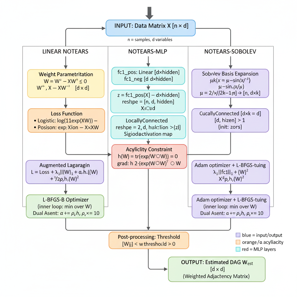
NOTEARS (“DAGs with NO TEARS”, Zheng et al., NeurIPS 2018) introduced a landmark reformulation of causal structure learning: instead of exhaustively searching the combinatorial space of \(2^{O(d^2)}\) possible directed acyclic graphs (an approach that becomes intractable for more than roughly ten variables), it recasts the problem as a smooth, gradient-based optimization over a real-valued weighted adjacency matrix \(\mathbf{W} \in \mathbb{R}^{d \times d}\).

Under the linear Structural Equation Model (SEM) assumption

\[\mathbf{X} = \mathbf{X}\mathbf{W} + \mathbf{Z},\]

where \(\mathbf{Z}\) contains independent noise terms (commonly Gaussian), the algorithm simultaneously (i) fits \(\mathbf{W}\) to the data via a reconstruction loss, (ii) enforces acyclicity through a closed-form differentiable constraint, and (iii) promotes sparsity with an \(\ell_1\) penalty.

Key innovation — the acyclicity constraint. The function

\[h(\mathbf{W}) = \mathrm{tr}\!\left(\exp(\mathbf{W} \odot \mathbf{W})\right) - d\]

equals zero if and only if the graph encoded by \(\mathbf{W}\) is acyclic. Because \(h\) is smooth and differentiable, the NP-hard combinatorial constraint is replaced by an equality constraint amenable to augmented Lagrangian (AL) optimization — no combinatorial search required.

NOTEARS is concise (the core algorithm fits in fewer than 60 lines of code), fast for moderate graph sizes (\(d \leq 100\)–\(200\)), and has become the canonical baseline against which all later continuous causal discovery methods are benchmarked — including GOLEM, DAG-GNN, and GraN-DAG.

NOTEARS with PyDeepCausalML

This notebook implements both the linear and nonlinear NOTEARS variants in Python using the PyDeepCausalML package. We apply them to synthetic data (linear and nonlinear SEMs) and evaluate performance against known ground-truth DAGs.

The PyDeepCausalML package encodes the full NOTEARS family. The acyclicity constraint \(h(W) = \mathrm{tr}(e^{W \odot W}) - d = 0\) is enforced via the trace of the matrix exponential, and optimization is handled by the augmented Lagrangian method with Adam inner steps.

Linear NOTEARS (NOTEARSLinear) learns a weighted adjacency matrix \(W\) by minimizing a least-squares loss plus an \(\ell_1\) penalty subject to \(h(W) = 0\).

Nonlinear NOTEARS (NOTEARSNonlinearMLP, NOTEARSNonlinearSobolev) replace the linear predictor with either an MLP or a Sobolev-basis model, allowing the algorithm to capture arbitrary smooth nonlinear relationships while keeping the same acyclicity constraint.

Main Classes

Class Role
NOTEARSLinear Linear NOTEARS: L2 loss + L1, augmented Lagrangian
NOTEARSNonlinearMLP Nonlinear NOTEARS with MLP per node
NOTEARSNonlinearSobolev Nonlinear NOTEARS with Sobolev / polynomial basis

Simulation and Evaluation Utilities

Function Role
is_dag Check whether a weighted adjacency matrix encodes a DAG
simulate_dag Simulate a random DAG (Erdős–Rényi or scale-free)
simulate_parameter Draw edge weights for a DAG
simulate_linear_sem Generate data from a linear SEM
simulate_nonlinear_sem_custom Generate data from a nonlinear SEM
count_accuracy / graph_recovery_metrics Compare estimated graph to ground truth

Reference: Zheng, X., Aragam, B., Ravikumar, P., & Xing, E. P. (2018). DAGs with NO TEARS: Continuous optimization for structure learning. NeurIPS. https://arxiv.org/abs/1803.01422.

Setup

Check and Install Required Python Packages

Code
import importlib
import subprocess
import sys

PACKAGES = [
    "numpy", "pandas", "scipy", "torch", "scikit-learn",
    "matplotlib", "seaborn", "networkx",
]

for pkg in PACKAGES:
    mod = "sklearn" if pkg == "scikit-learn" else pkg
    try:
        importlib.import_module(mod)
    except ImportError:
        subprocess.check_call([sys.executable, "-m", "pip", "install", "-q", pkg])

try:
    import pydeepcausalml  # noqa: F401
except ImportError:
    subprocess.check_call(
        [sys.executable, "-m", "pip", "install", "-q",
         "git+https://github.com/zia207/PyDeepCausalML.git"]
    )

import pydeepcausalml
print("pydeepcausalml", pydeepcausalml.__version__, "ready.")
pydeepcausalml 0.2.0 ready.

Verify imports

Code
import numpy as np
import pandas as pd
import torch
import matplotlib.pyplot as plt
import seaborn as sns
import networkx as nx
from sklearn.linear_model import LinearRegression

from pydeepcausalml import set_seed
from pydeepcausalml.metrics import graph_recovery_metrics, shd, pehe

print("torch:", torch.__version__)
print("cuda:", torch.cuda.is_available())
torch: 2.12.1+cu130
cuda: False
Code
set_seed(42)
run_fast = True

Simulation utilities

Code
"""Simulation and evaluation helpers (NOTEARS tutorial utilities)."""

def is_dag(W: np.ndarray, tol: float = 1e-8) -> bool:
    """Return True if weighted matrix W encodes a DAG."""
    d = W.shape[0]
    m = (np.abs(W) > tol).astype(float)
    acc = m.copy()
    for _ in range(d):
        if np.trace(acc) > tol:
            return False
        acc = acc @ m
    return True


def simulate_dag(d: int, s0: int, graph_type: str = "ER", seed: int | None = None) -> np.ndarray:
    """Simulate a random binary DAG adjacency (A[i,j]=1 => X_j -> X_i)."""
    rng = np.random.default_rng(seed)
    if graph_type.upper() == "ER":
        prob = min(1.0, s0 / max(d * (d - 1) / 2, 1))
        B = np.triu(rng.random((d, d)) < prob, k=1).astype(int)
    else:  # scale-free-ish upper triangular
        B = np.zeros((d, d), dtype=int)
        edges = 0
        while edges < s0:
            i, j = rng.integers(0, d, size=2)
            if i < j and B[i, j] == 0:
                B[i, j] = 1
                edges += 1
    return B


def simulate_parameter(B: np.ndarray, low: float = 0.5, high: float = 2.0, seed: int | None = None) -> np.ndarray:
    """Draw edge weights for a binary DAG."""
    rng = np.random.default_rng(seed)
    W = np.zeros_like(B, dtype=float)
    mask = B.astype(bool)
    signs = rng.choice([-1.0, 1.0], size=mask.sum())
    W[mask] = signs * rng.uniform(low, high, size=mask.sum())
    return W


def simulate_linear_sem(W: np.ndarray, n: int, sem_type: str = "gauss", seed: int | None = None) -> np.ndarray:
    """Generate data from a linear SEM in topological order.

    With an upper-triangular weight matrix ``W`` (``W[i, j] != 0`` means
    ``X_i -> X_j``), each node is drawn as ``X_j = sum_i W[i, j] X_i + Z_j``.
    Sampling node-by-node in index order is exact here because parents always
    have a smaller index than their children.
    """
    rng = np.random.default_rng(seed)
    d = W.shape[0]
    X = np.zeros((n, d))
    for j in range(d):
        parents = np.where(W[:, j] != 0)[0]
        noise = rng.standard_normal(n) if sem_type == "gauss" else rng.exponential(size=n)
        if len(parents):
            X[:, j] = X[:, parents] @ W[parents, j] + noise
        else:
            X[:, j] = noise
    return X


def count_accuracy(B_true: np.ndarray, B_est: np.ndarray) -> dict:
    """Compare estimated graph to ground truth (FDR, TPR, FPR, SHD, nnz)."""
    m = graph_recovery_metrics(B_true, B_est)
    tp, fp, fn = m["tp"], m["fp"], m["fn"]
    tn = int((~np.eye(B_true.shape[0], dtype=bool)).sum()) - tp - fp - fn
    fdr = fp / (tp + fp) if tp + fp else 0.0
    tpr = m["recall"]
    fpr = fp / (fp + tn) if fp + tn else 0.0
    return {"fdr": fdr, "tpr": tpr, "fpr": fpr, "shd": m["shd"], "nnz": int(B_est.sum())}


def simulate_nonlinear_sem_custom(W: np.ndarray, n: int, sem_type: str = "mlp", noise_sd: float = 0.5, seed: int | None = None) -> np.ndarray:
    """Nonlinear SEM with additive noise (A[i,j]: j->i)."""
    rng = np.random.default_rng(seed)
    d = W.shape[0]
    G = nx.DiGraph((j, i) for i in range(d) for j in range(d) if W[i, j] != 0)
    order = list(nx.topological_sort(G)) if G.number_of_edges() else list(range(d))
    X = np.zeros((n, d))
    for i in order:
        pa = np.where(W[i, :] != 0)[0]
        if len(pa) == 0:
            X[:, i] = rng.standard_normal(n)
        else:
            z = X[:, pa] @ W[i, pa]
            if sem_type == "mlp":
                X[:, i] = np.tanh(z) + rng.normal(0, noise_sd, n)
            elif sem_type == "mim":
                X[:, i] = z * np.sin(z) + rng.normal(0, noise_sd, n)
            elif sem_type == "gp":
                X[:, i] = np.sin(z) + rng.normal(0, noise_sd, n)
            else:
                X[:, i] = z + rng.standard_normal(n)
    return X

Part I: Linear NOTEARS on Synthetic Gaussian Data

Overview

We begin with a linear Gaussian SEM: variables are generated by the model \(\mathbf{X} = \mathbf{X}\mathbf{W} + \mathbf{Z}\), where \(\mathbf{Z} \sim \mathcal{N}(0, I)\). The ground-truth DAG is known, so we can measure recovery accuracy precisely.

Data Generation and Preprocessing

Code
# Dataset 1: Linear Gaussian SEM (d = 20)
set_seed(42)

n_lin, d_lin, s0_lin = 2000, 20, 20
graph_type, sem_type_lin = "ER", "gauss"

B_true_lin = simulate_dag(d_lin, s0_lin, graph_type, seed=42)
W_true_lin = simulate_parameter(B_true_lin, seed=42)
X_lin = simulate_linear_sem(W_true_lin, n_lin, sem_type_lin, seed=42)

# Center columns — NOTEARS is sensitive to variable scale
X_lin = X_lin - X_lin.mean(axis=0, keepdims=True)

rng = np.random.default_rng(42)
idx = rng.permutation(n_lin)
tr1 = idx[: int(0.70 * n_lin)]
tmp1 = idx[int(0.70 * n_lin) :]
va1 = tmp1[: len(tmp1) // 2]
te1 = tmp1[len(tmp1) // 2 :]

X_lin_train, X_lin_val, X_lin_test = X_lin[tr1], X_lin[va1], X_lin[te1]
print("Linear SEM — Train:", X_lin_train.shape, "| Val:", X_lin_val.shape, "| Test:", X_lin_test.shape)
Linear SEM — Train: (1400, 20) | Val: (300, 20) | Test: (300, 20)

Fitting Linear NOTEARS

The algorithm minimizes the augmented Lagrangian

\[\mathcal{L}_\rho(W, \alpha) = \frac{1}{2n}\|X - XW\|_F^2 + \lambda_1\|W\|_1 + \alpha\, h(W) + \frac{\rho}{2}h(W)^2,\]

iterating (i) gradient steps on \(W\) and (ii) dual-ascent updates until \(h(W) < \epsilon\).

Code
from pydeepcausalml.discovery import NOTEARSLinear

model_lin = NOTEARSLinear(
    lambda_l1=0.05,
    epochs=100,
    n_outer=100,
    lr=1e-2,
    random_state=42,
)
model_lin.fit(X_lin_train)

W_est_lin = model_lin.weights_
w_threshold = 0.3
B_est_lin = model_lin.get_adjacency(threshold=w_threshold)

print("Acyclic (thresholded, linear SEM):", is_dag(B_est_lin))
n_val_lin = X_lin_val.shape[0]
val_loss_lin = 0.5 / n_val_lin * np.sum((X_lin_val - X_lin_val @ W_est_lin.T) ** 2)
print(f"Validation L2 loss (linear model | linear SEM): {val_loss_lin:.6f}")
Acyclic (thresholded, linear SEM): True
Validation L2 loss (linear model | linear SEM): 25.046984

Hyperparameter guidance. The two most impactful choices are: (i) the sparsity penalty \(\lambda_1 \in [0.01, 0.5]\) — higher values prune more edges; and (ii) the edge-threshold \(w_{\mathrm{threshold}} \in [0.1, 0.5]\) applied after optimization.

Causal Effect Estimation via Backdoor Adjustment

NOTEARS recovers graph structure, not causal effects directly. Once the DAG is in hand, downstream causal inference proceeds in two steps: (i) read off a valid adjustment set from the graph using the backdoor criterion, and (ii) estimate the Average Treatment Effect (ATE) by regression on that set.

The example below treats variable 0 as the treatment \(T\) and variable 19 as the outcome \(Y\) (0-indexed).

Code
# True ATE via structural path sum: (I - W)^{-1}[Y, T]
I_lin = np.eye(d_lin)
true_total_lin = np.linalg.solve(I_lin - W_true_lin, np.eye(d_lin))
true_ATE_lin = true_total_lin[19, 0]
print(f"True ATE (T -> Y, linear SEM):  {true_ATE_lin:.4f}")

confounders_idx_lin = [i for i in range(d_lin) if i not in (0, 19)]
T_tr_lin = X_lin_train[:, 0:1]
Y_tr_lin = X_lin_train[:, 19]
C_tr_lin = X_lin_train[:, confounders_idx_lin]

model_ate_lin = LinearRegression().fit(np.hstack([T_tr_lin, C_tr_lin]), Y_tr_lin)
est_ATE_lin = model_ate_lin.coef_[0]
print(f"Estimated ATE:  {est_ATE_lin:.4f}  (error: {abs(est_ATE_lin - true_ATE_lin):.4f})")
True ATE (T -> Y, linear SEM):  0.0000
Estimated ATE:  -0.0539  (error: 0.0539)

Graph Recovery Metrics

When the ground-truth DAG is known, five complementary metrics quantify structural recovery accuracy.

  • FDR — fraction of predicted edges that are spurious.
  • TPR (Recall) — fraction of true edges recovered.
  • FPR — fraction of true non-edges incorrectly predicted.
  • SHD — edge insertions + deletions to match the true graph.
  • nnz — number of edges in the estimated graph.
Code
acc_lin_result = count_accuracy(B_true_lin, B_est_lin)
print(acc_lin_result)
{'fdr': 0.6153846153846154, 'tpr': 0.2941, 'fpr': 0.02203856749311295, 'shd': 20, 'nnz': 13}

Visualization

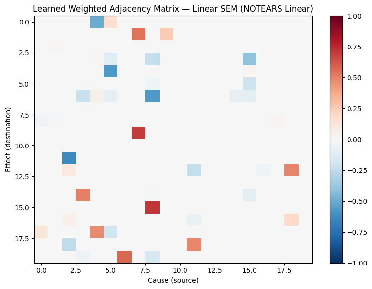
Weighted Adjacency Matrix

Code
fig, ax = plt.subplots(figsize=(8, 6))
im = ax.imshow(W_est_lin, cmap="RdBu_r", vmin=-1, vmax=1, aspect="auto")
ax.set_title("Learned Weighted Adjacency Matrix — Linear SEM (NOTEARS Linear)")
ax.set_xlabel("Cause (source)")
ax.set_ylabel("Effect (destination)")
plt.colorbar(im, ax=ax)
plt.tight_layout()
plt.show()

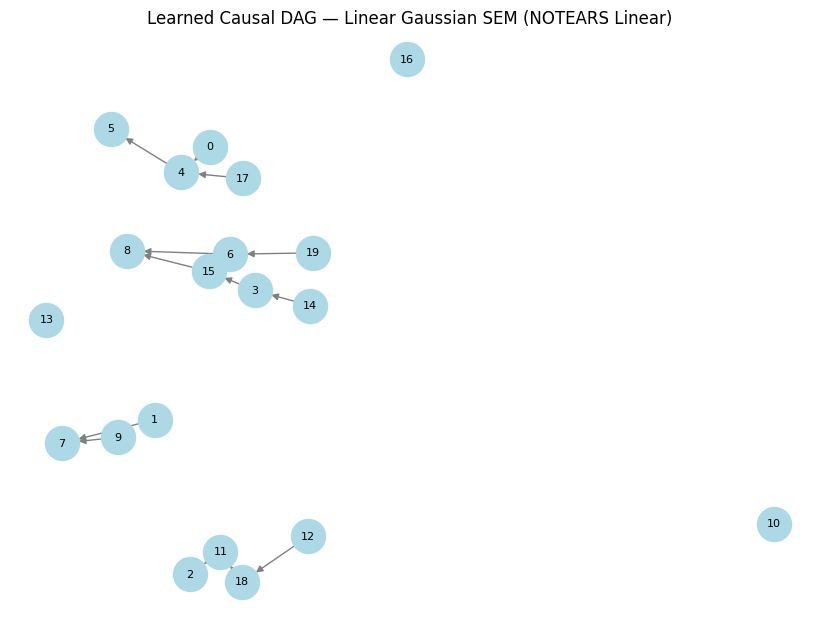
Learned Causal DAG

Code
G_lin = nx.from_numpy_array((np.abs(W_est_lin) > w_threshold).astype(int), create_using=nx.DiGraph)
pos_lin = nx.spring_layout(G_lin, seed=42)
plt.figure(figsize=(8, 6))
nx.draw(G_lin, pos_lin, with_labels=True, node_color="lightblue", arrows=True,
        node_size=600, font_size=8, edge_color="gray")
plt.title("Learned Causal DAG — Linear Gaussian SEM (NOTEARS Linear)")
plt.show()


Part II: Nonlinear NOTEARS (MLP and Sobolev) vs. Misspecified Baseline

Overview

We now stress-test the linear model on data generated from a nonlinear SEM and compare it against two nonlinear NOTEARS variants.

Code
# Dataset 2: Nonlinear SEM (d = 10)
set_seed(42)
n_nlin, d_nlin, s0_nlin = 2000, 10, 10
B_true_nlin = simulate_dag(d_nlin, s0_nlin, graph_type, seed=42)
W_true_nlin = simulate_parameter(B_true_nlin, seed=42)
X_nlin = simulate_nonlinear_sem_custom(W_true_nlin, n_nlin, sem_type="mlp", seed=42)
X_nlin = X_nlin - X_nlin.mean(axis=0, keepdims=True)

rng = np.random.default_rng(42)
idx = rng.permutation(n_nlin)
tr2 = idx[: int(0.70 * n_nlin)]
tmp2 = idx[int(0.70 * n_nlin) :]
va2 = tmp2[: len(tmp2) // 2]
te2 = tmp2[len(tmp2) // 2 :]
X_nlin_train, X_nlin_val, X_nlin_test = X_nlin[tr2], X_nlin[va2], X_nlin[te2]
print("Nonlinear SEM — Train:", X_nlin_train.shape, "| Val:", X_nlin_val.shape, "| Test:", X_nlin_test.shape)
Nonlinear SEM — Train: (1400, 10) | Val: (300, 10) | Test: (300, 10)

Model 1: Linear NOTEARS (Misspecified Baseline)

Code
model_lin_nl = NOTEARSLinear(lambda_l1=0.1, epochs=100, n_outer=100, random_state=42)
model_lin_nl.fit(X_nlin_train)
W_lin_nlin = model_lin_nl.weights_
B_lin_nlin = model_lin_nl.get_adjacency(threshold=0.3)
print("Linear NOTEARS on nonlinear SEM — acyclic:", is_dag(B_lin_nlin))
n_val_nlin = X_nlin_val.shape[0]
val_loss_lin_nl = 0.5 / n_val_nlin * np.sum((X_nlin_val - X_nlin_val @ W_lin_nlin.T) ** 2)
print(f"Validation L2 loss (linear model | nonlinear SEM): {val_loss_lin_nl:.6f}")
Linear NOTEARS on nonlinear SEM — acyclic: True
Validation L2 loss (linear model | nonlinear SEM): 2.599821

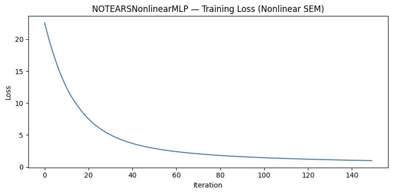
Model 2: NOTEARSNonlinearMLP

Code
from pydeepcausalml.discovery import NOTEARSNonlinearMLP, NOTEARSNonlinearSobolev

set_seed(42)
model_mlp = NOTEARSNonlinearMLP(hidden=10, lambda1=0.01, rho=1.0, epochs=150, lr=1e-2, random_state=42)
model_mlp.fit(X_nlin_train)
W_mlp_nlin = model_mlp.adjacency_matrix()
B_mlp_nlin = (W_mlp_nlin > 1e-5).astype(int)
print("NOTEARSNonlinearMLP on nonlinear SEM — acyclic:", is_dag(B_mlp_nlin))

if model_mlp.history_.get("loss"):
    plt.figure(figsize=(8, 4))
    plt.plot(model_mlp.history_["loss"], color="steelblue")
    plt.title("NOTEARSNonlinearMLP — Training Loss (Nonlinear SEM)")
    plt.xlabel("Iteration")
    plt.ylabel("Loss")
    plt.tight_layout()
    plt.show()
NOTEARSNonlinearMLP on nonlinear SEM — acyclic: False

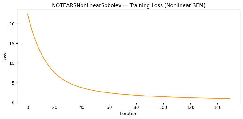
Model 3: NOTEARSNonlinearSobolev

Code
set_seed(42)
model_sob = NOTEARSNonlinearSobolev(degree=4, lambda1=0.01, rho=1.0, epochs=150, lr=1e-2, random_state=42)
model_sob.fit(X_nlin_train)
W_sob_nlin = model_sob.adjacency_matrix()
B_sob_nlin = (W_sob_nlin > 1e-5).astype(int)
print("NOTEARSNonlinearSobolev on nonlinear SEM — acyclic:", is_dag(B_sob_nlin))

if model_sob.history_.get("loss"):
    plt.figure(figsize=(8, 4))
    plt.plot(model_sob.history_["loss"], color="darkorange")
    plt.title("NOTEARSNonlinearSobolev — Training Loss (Nonlinear SEM)")
    plt.xlabel("Iteration")
    plt.ylabel("Loss")
    plt.tight_layout()
    plt.show()
NOTEARSNonlinearSobolev on nonlinear SEM — acyclic: False

Model Comparison

Code
def safe_acc(B_true, W_est, B_est, label):
    if not is_dag(W_est):
        print(f"  {label:30s}  NOT a DAG — skipping metrics")
        return None
    return count_accuracy(B_true, B_est)

acc_lin_on_nlin = safe_acc(B_true_nlin, W_lin_nlin, B_lin_nlin, "Linear NOTEARS (nonlin SEM)")
acc_mlp_on_nlin = safe_acc(B_true_nlin, W_mlp_nlin, B_mlp_nlin, "NOTEARSNonlinearMLP")
acc_sob_on_nlin = safe_acc(B_true_nlin, W_sob_nlin, B_sob_nlin, "NOTEARSNonlinearSobolev")

def print_row(label, acc):
    if acc is None:
        print(f"  {label:34s} {'--':>7s} {'--':>7s} {'--':>7s} {'--':>5s} {'--':>5s}")
    else:
        print(f"  {label:34s} {acc['fdr']:7.4f} {acc['tpr']:7.4f} {acc['fpr']:7.4f} {acc['shd']:5d} {acc['nnz']:5d}")

div = "-" * 72
print("\n", div)
print(f"  {'Model':34s} {'FDR':>7s} {'TPR':>7s} {'FPR':>7s} {'SHD':>5s} {'nnz':>5s}")
print(div)
print(f"  {'Linear NOTEARS — native SEM *':34s} {acc_lin_result['fdr']:7.4f} {acc_lin_result['tpr']:7.4f} {acc_lin_result['fpr']:7.4f} {acc_lin_result['shd']:5d} {acc_lin_result['nnz']:5d}   (d=20, linear SEM)")
print(div)
print_row("Linear NOTEARS  (misspecified baseline)", acc_lin_on_nlin)
print_row("NOTEARSNonlinearMLP (hidden=10)", acc_mlp_on_nlin)
print_row("NOTEARSNonlinearSobolev (degree=4)", acc_sob_on_nlin)
print(div)
print(f"  True edges in nonlinear SEM graph: {int(B_true_nlin.sum())}  |  d = {d_nlin}")
  Linear NOTEARS (nonlin SEM)     NOT a DAG — skipping metrics
  NOTEARSNonlinearMLP             NOT a DAG — skipping metrics
  NOTEARSNonlinearSobolev         NOT a DAG — skipping metrics

 ------------------------------------------------------------------------
  Model                                  FDR     TPR     FPR   SHD   nnz
------------------------------------------------------------------------
  Linear NOTEARS — native SEM *       0.6154  0.2941  0.0220    20    13   (d=20, linear SEM)
------------------------------------------------------------------------
  Linear NOTEARS  (misspecified baseline)      --      --      --    --    --
  NOTEARSNonlinearMLP (hidden=10)         --      --      --    --    --
  NOTEARSNonlinearSobolev (degree=4)      --      --      --    --    --
------------------------------------------------------------------------
  True edges in nonlinear SEM graph: 12  |  d = 10

ATE Estimation on the Nonlinear SEM

Code
T_idx_nlin, Y_idx_nlin = 0, d_nlin - 1

if acc_mlp_on_nlin is not None:
    W_best_nlin, label_best = W_mlp_nlin, "NOTEARSNonlinearMLP"
elif acc_sob_on_nlin is not None:
    W_best_nlin, label_best = W_sob_nlin, "NOTEARSNonlinearSobolev"
else:
    W_best_nlin, label_best = W_lin_nlin, "Linear NOTEARS (fallback)"
print(f"Adjustment set derived from: {label_best}")

pa_Y_nlin = np.where(np.abs(W_best_nlin[Y_idx_nlin, :]) > 1e-5)[0]
conf_nlin = [i for i in pa_Y_nlin if i != T_idx_nlin]
if not conf_nlin:
    conf_nlin = [i for i in range(d_nlin) if i not in (T_idx_nlin, Y_idx_nlin)]

T_n = X_nlin_train[:, T_idx_nlin:T_idx_nlin + 1]
Y_n = X_nlin_train[:, Y_idx_nlin]
C_n = X_nlin_train[:, conf_nlin]

X_design = np.hstack([T_n, C_n])
model_ate_nlin = LinearRegression().fit(X_design, Y_n)
ate_nlin = model_ate_nlin.coef_[0]
ate_unadj_nlin = LinearRegression().fit(T_n, Y_n).coef_[0]

rng = np.random.default_rng(42)
ate_boot = []
for _ in range(500):
    idx = rng.integers(0, X_nlin_train.shape[0], X_nlin_train.shape[0])
    Tb = X_nlin_train[idx, T_idx_nlin:T_idx_nlin + 1]
    Yb = X_nlin_train[idx, Y_idx_nlin]
    Cb = X_nlin_train[np.ix_(idx, conf_nlin)]
    ate_boot.append(LinearRegression().fit(np.hstack([Tb, Cb]), Yb).coef_[0])
ci_lo, ci_hi = np.quantile(ate_boot, [0.025, 0.975])

try:
    struct_ate = np.linalg.solve(np.eye(d_nlin) - W_best_nlin, np.eye(d_nlin))[Y_idx_nlin, T_idx_nlin]
except np.linalg.LinAlgError:
    struct_ate = np.nan

print(f"\nATE  (T={T_idx_nlin} -> Y={Y_idx_nlin})  on Nonlinear SEM")
print(f"  Adjusted estimate   : {ate_nlin:+.4f}")
print(f"  Unadjusted estimate : {ate_unadj_nlin:+.4f}")
print(f"  Bootstrap 95% CI    : [{ci_lo:.4f}, {ci_hi:.4f}]")
print(f"  Structural ATE (W)  : {struct_ate:+.4f}  (linear approx.)")
Adjustment set derived from: Linear NOTEARS (fallback)

ATE  (T=0 -> Y=9)  on Nonlinear SEM
  Adjusted estimate   : -0.0194
  Unadjusted estimate : +0.3643
  Bootstrap 95% CI    : [-0.0701, 0.0309]
  Structural ATE (W)  : +0.0015  (linear approx.)

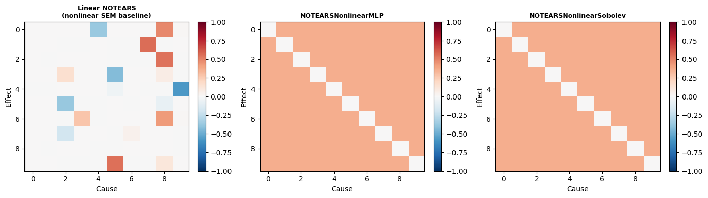
Visualization — Adjacency Matrix Heatmaps

Code
def make_heatmap(W, title_str, lim=1.0):
    fig, ax = plt.subplots(figsize=(4.5, 4))
    im = ax.imshow(W, cmap="RdBu_r", vmin=-lim, vmax=lim, aspect="auto")
    ax.set_title(title_str, fontsize=9, fontweight="bold")
    ax.set_xlabel("Cause")
    ax.set_ylabel("Effect")
    plt.colorbar(im, ax=ax, fraction=0.046)
    return fig

fig, axes = plt.subplots(1, 3, figsize=(14, 4))
for ax, W, title in zip(
    axes,
    [W_lin_nlin, W_mlp_nlin, W_sob_nlin],
    ["Linear NOTEARS\n(nonlinear SEM baseline)", "NOTEARSNonlinearMLP", "NOTEARSNonlinearSobolev"],
):
    im = ax.imshow(W, cmap="RdBu_r", vmin=-1, vmax=1, aspect="auto")
    ax.set_title(title, fontsize=9, fontweight="bold")
    ax.set_xlabel("Cause")
    ax.set_ylabel("Effect")
    plt.colorbar(im, ax=ax, fraction=0.046)
plt.tight_layout()
plt.show()

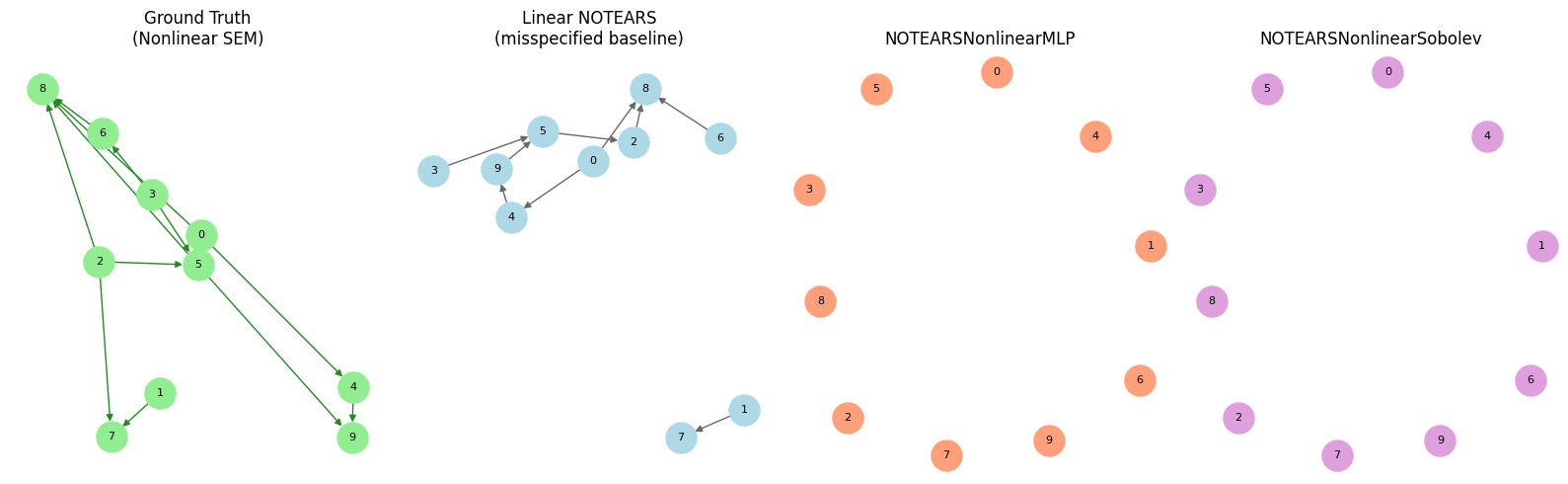
Visualization — Learned DAGs

Code
fig, axes = plt.subplots(1, 4, figsize=(16, 5))

def plot_dag_ax(ax, B, title, node_color="lightblue", edge_color="dimgray"):
    G = nx.from_numpy_array(B.astype(int), create_using=nx.DiGraph)
    pos = nx.spring_layout(G, seed=42)
    nx.draw(G, pos, ax=ax, with_labels=True, node_color=node_color, edge_color=edge_color,
            arrows=True, node_size=500, font_size=8)
    ax.set_title(title)

plot_dag_ax(axes[0], B_true_nlin, "Ground Truth\n(Nonlinear SEM)", "lightgreen", "forestgreen")
plot_dag_ax(axes[1], B_lin_nlin, "Linear NOTEARS\n(misspecified baseline)")
B_plot_mlp = B_mlp_nlin if acc_mlp_on_nlin else np.zeros((d_nlin, d_nlin))
B_plot_sob = B_sob_nlin if acc_sob_on_nlin else np.zeros((d_nlin, d_nlin))
plot_dag_ax(axes[2], B_plot_mlp, "NOTEARSNonlinearMLP", "lightsalmon", "tomato")
plot_dag_ax(axes[3], B_plot_sob, "NOTEARSNonlinearSobolev", "plum", "purple")
plt.tight_layout()
plt.show()

Interpretation

Linear NOTEARS on nonlinear data is a deliberate stress test. Nonlinear variants tend to outperform when sample size is sufficient (\(n \geq 500\) per variable).

DAG validity must be verified with is_dag() before interpreting any structural metric.

Summary and Conclusion

NOTEARS transformed causal structure learning by replacing an NP-hard combinatorial search with a smooth continuous optimization problem.

Strengths. The linear variant is simple, fast on moderate graphs (\(d \leq 200\)), and produces interpretable weighted edges.

Limitations. The linear variant assumes additive Gaussian noise with no hidden confounders. Always center or standardize variables before fitting.

Resources

Back to top