Python Banner

4.4 Double ML with Instrumental Variables

DML-IV combines an instrument with cross-fitted nuisance models. The instrument \(Z\) addresses endogeneity of the treatment \(D\). Machine learning partials observed covariates out of \(Y\), \(D\), and \(Z\). The final regression of outcome residuals on treatment residuals, using the instrument residuals as the instrument, is a cross-fitted cousin of two-stage least squares.

Overview

Node Role
\(Z\) Instrument: affects \(D\), and affects \(Y\) only through \(D\)
\(C\) Unobserved confounder
\(D\) Endogenous treatment
\(Y\) Outcome

A regression of \(Y\) on \(D\) is biased when \(C\) moves both. Partial linear DML without an instrument does not remove that bias. DML-IV does, under the usual IV assumptions (relevance, exclusion, and independence of \(Z\) given the observed covariates).

With covariates \(W\), the partially linear IV score residualizes all three variables:

\[\tilde Y = Y - \hat E[Y\mid W], \quad \tilde D = D - \hat E[D\mid W], \quad \tilde Z = Z - \hat E[Z\mid W]\]

\[\hat\theta = \frac{\sum_i \tilde Z_i \tilde Y_i}{\sum_i \tilde Z_i \tilde D_i}.\]

InstrumentalVariable in PyCausalML is the linear two-stage least squares version of the same idea, with a Bayesian bootstrap interval. PartiallyLinearDML is the no-instrument comparison.

Implementation in Python

  1. Simulate (Part A) or load (Part B) the sample.
  2. Pass observed covariates into the nuisance regressions so a forest has something to split on.
  3. Compute the naive mean difference.
  4. Fit DML-IV and PartiallyLinearDML for ridge, random-forest, and gradient-boosting nuisances.
  5. Compare estimates with the known effect in Part A, and across learners in Part B.

Data/data_401k.csv records eligibility (e401) and net financial assets, which is the partially linear 401(k) design. It does not contain a separate participation indicator, so the instrumental-variables contrast — eligibility as an instrument for an endogenous decision — is identified in the simulation, where \(Z\), \(D\), and \(C\) are all generated. Part B estimates the eligibility effect on the real file and explains a linear CATE with SHAP.

Set Up

Code
import subprocess
import sys
from pathlib import Path

def _repo_root() -> Path:
    here = Path.cwd().resolve()
    for cand in [here, *here.parents]:
        if (cand / "pyproject.toml").is_file() and (cand / "src" / "pycausalml").is_dir():
            return cand
    raise FileNotFoundError(
        "PyCausalML repository was not found. Run this notebook from the repository."
    )

root = _repo_root()
data_dir = root / "Data"
if not data_dir.is_dir():
    raise FileNotFoundError(
        "The Data directory was not found. It should sit next to pyproject.toml."
    )

try:
    import pycausalml  # noqa: F401
    print("PyCausalML ready.")
except ImportError:
    subprocess.check_call(
        [sys.executable, "-m", "pip", "install", "-q", "-e", f"{root}[plot]"],
    )
    print("PyCausalML installed.")
print("Data directory:", data_dir)
PyCausalML ready.
Data directory: /home/zia207/Github/PyCausalML/Data
Code
%matplotlib inline
import matplotlib.pyplot as plt
import numpy as np
import pandas as pd
from scipy import stats
from sklearn.ensemble import (
    GradientBoostingClassifier,
    GradientBoostingRegressor,
    RandomForestClassifier,
    RandomForestRegressor,
)
from sklearn.linear_model import Lasso, LassoCV, LogisticRegression, Ridge
from sklearn.metrics import (
    accuracy_score,
    average_precision_score,
    brier_score_loss,
    mean_squared_error,
    precision_recall_curve,
    roc_auc_score,
    roc_curve,
)
from sklearn.model_selection import KFold
from sklearn.pipeline import Pipeline
from sklearn.preprocessing import PolynomialFeatures, StandardScaler

from pycausalml import (
    CausalForestDML,
    InteractiveRegressionDML,
    KernelDML,
    LinearDML,
    NonParamDML,
    PartiallyLinearDML,
    SparseLinearDML,
    explain_cate,
)
from pycausalml.interpretation import plot_cate_hist

plt.rcParams["figure.dpi"] = 110
print("Imported PyCausalML")

from pycausalml import InstrumentalVariable
Imported PyCausalML
Code
def cross_fit_predict(X, y, n_splits, seed, kind="ridge"):
    """Out-of-fold predictions. kind is 'ridge', 'rf', or 'gbr'."""
    pred = np.zeros(len(y), dtype=float)
    splitter = KFold(n_splits=n_splits, shuffle=True, random_state=seed)
    y = np.asarray(y, dtype=float)
    for fold, (tr, te) in enumerate(splitter.split(X)):
        model = _nuisance(kind, seed + fold)
        model.fit(X[tr], y[tr])
        pred[te] = model.predict(X[te])
    return pred


def _nuisance(kind, seed):
    if kind == "ridge":
        return Ridge(alpha=1.0)
    if kind == "lasso":
        return Lasso(alpha=0.02, max_iter=8000)
    if kind == "rf":
        return RandomForestRegressor(
            n_estimators=40, max_depth=4, min_samples_leaf=5, random_state=seed, n_jobs=1,
        )
    if kind == "gbr":
        return GradientBoostingRegressor(
            n_estimators=40, max_depth=2, learning_rate=0.08, random_state=seed,
        )
    raise ValueError(kind)


def plot_beeswarm(explanation, title, max_display=8):
    imp = explanation.importance()
    order = np.argsort(imp)[-max_display:]
    fig, ax = plt.subplots(figsize=(7.2, 0.42 * len(order) + 1.3))
    rng = np.random.default_rng(0)
    for i, j in enumerate(order):
        vals = explanation.values[:, j]
        raw = explanation.data[:, j]
        span = float(np.ptp(raw)) or 1.0
        color = (raw - np.min(raw)) / span
        jitter = rng.uniform(-0.16, 0.16, size=len(vals))
        ax.scatter(vals, np.full(len(vals), i) + jitter, c=color, cmap="coolwarm", s=18, alpha=0.9)
    ax.set_yticks(np.arange(len(order)))
    ax.set_yticklabels([explanation.feature_names[j] for j in order])
    ax.axvline(0, color="grey", lw=0.8)
    ax.set_xlabel("SHAP value")
    ax.set_title(title)
    fig.tight_layout()
    return fig


print("Helpers ready")
Helpers ready
Code
def dml_iv(W, d, z, y, kind="ridge", n_splits=3, seed=0):
    y_res = y - cross_fit_predict(W, y, n_splits, seed, kind)
    d_res = d - cross_fit_predict(W, d, n_splits, seed + 3, kind)
    z_res = z - cross_fit_predict(W, z, n_splits, seed + 6, kind)
    denom = float(np.dot(z_res, d_res))
    theta = float(np.dot(z_res, y_res) / denom)
    psi = z_res * (y_res - theta * d_res) / np.mean(z_res * d_res)
    se = float(np.std(psi, ddof=1) / np.sqrt(len(psi)))
    return theta, se


class IVLinearCATE:
    """Linear CATE from a cross-fitted IV score, for SHAP."""

    def __init__(self, kind="ridge", n_splits=2, seed=0):
        self.kind = kind
        self.n_splits = n_splits
        self.seed = seed

    def fit(self, X, d, z, y, feature_names=None):
        X = np.asarray(X, dtype=float)
        y_res = y - cross_fit_predict(X, y, self.n_splits, self.seed, self.kind)
        d_res = d - cross_fit_predict(X, d, self.n_splits, self.seed + 3, self.kind)
        z_res = z - cross_fit_predict(X, z, self.n_splits, self.seed + 6, self.kind)
        phi = np.column_stack([np.ones(len(X)), X])
        design = z_res[:, None] * phi
        # Project y_res onto the instrumented treatment interacted with phi.
        # Use d_res on the left of the normal equations via 2SLS-style scaling:
        # solve (Zphi' Dphi) beta = Zphi' y, with Dphi = d_res * phi.
        d_design = d_res[:, None] * phi
        beta, *_ = np.linalg.lstsq(design.T @ d_design, design.T @ y_res, rcond=None)
        self.intercept_ = float(beta[0])
        self.feature_coef_ = np.asarray(beta[1:], dtype=float)
        self.feature_names_ = list(feature_names) if feature_names is not None else [f"x{j}" for j in range(X.shape[1])]
        return self

    def predict(self, X):
        X = np.asarray(X, dtype=float)
        return self.intercept_ + X @ self.feature_coef_

    predict_cate = predict


print("IV helpers ready")

IV helpers ready

Part A: DML-IV with Synthetic Data

Data-generating process

  • \(C\): binary unobserved confounder
  • \(Z\): binary instrument
  • \(D\): binary decision, increasing in \(Z\) and in \(C\)
  • \(Y\): continuous outcome. The structural effect of \(D\) is \(-2\)
  • \(W\): three noise covariates passed to the nuisance models

The naive difference in means is pulled upward by \(C\).

Code
def make_iv_sample(n=4000, seed=0):
    rng = np.random.default_rng(seed)
    confounder = rng.binomial(1, 0.5, size=n).astype(float)
    instrument = rng.binomial(1, 0.5, size=n).astype(float)
    covariates = rng.normal(size=(n, 3))
    logits = -0.4 + 1.6 * instrument + 1.7 * confounder
    propensity = 1.0 / (1.0 + np.exp(-logits))
    decision = rng.binomial(1, propensity).astype(float)
    outcome = -2.0 * decision + 4.0 * confounder + 0.15 * covariates[:, 0] + rng.normal(size=n)
    return covariates, instrument, decision, outcome


W, Z, D, Y = make_iv_sample()
naive = float(Y[D == 1].mean() - Y[D == 0].mean())
print("Naive mean difference:", round(naive, 3), "(true effect is -2)")
Naive mean difference: -0.497 (true effect is -2)

The naive estimate is far from \(-2\). Units with \(C = 1\) are both more likely to take the decision and have a higher baseline outcome.

DML-IV versus standard DML

Code
rows = [{"Estimator": "Naive mean difference", "Learner": "—", "Estimate": naive, "Std. err": np.nan}]
for kind in ("ridge", "rf", "gbr"):
    theta, se = dml_iv(W, D, Z, Y, kind=kind, seed=20)
    rows.append({"Estimator": "DML-IV", "Learner": kind, "Estimate": theta, "Std. err": se})
    plr = PartiallyLinearDML(
        discrete_treatment=True, n_splits=3, model_y=kind if kind != "gbr" else "gbr",
        n_estimators=40, random_state=20,
    )
    plr.fit(W, D, Y, feature_names=["W1", "W2", "W3"])
    summary = plr.average_treatment_effect()
    rows.append({
        "Estimator": "PartiallyLinearDML (no instrument)",
        "Learner": kind,
        "Estimate": summary["estimate"],
        "Std. err": summary["std.err"],
    })
comparison = pd.DataFrame(rows)
comparison.round(3)
Estimator Learner Estimate Std. err
0 Naive mean difference — -0.497 NaN
1 DML-IV ridge -1.767 0.247
2 PartiallyLinearDML (no instrument) ridge -0.497 0.071
3 DML-IV rf -1.763 0.247
4 PartiallyLinearDML (no instrument) rf -0.494 0.071
5 DML-IV gbr -1.785 0.247
6 PartiallyLinearDML (no instrument) gbr -0.501 0.071

Takeaway. For every first-stage learner, DML-IV recovers a value near the structural effect of \(-2\). PartiallyLinearDML has no instrument, so it stays near the confounded naive contrast.

Minimal reference fit

Linear nuisances, and InstrumentalVariable (two-stage least squares) on the same sample.

Code
theta_ref, se_ref = dml_iv(W, D, Z, Y, kind="ridge", n_splits=5, seed=1)
iv_linear = InstrumentalVariable(n_boot=80, random_state=1)
iv_linear.fit(Y, D, Z, X=W)
print("DML-IV ridge:", round(theta_ref, 3), "se", round(se_ref, 3))
print("InstrumentalVariable:", iv_linear.summary())
DML-IV ridge: -1.778 se 0.247
InstrumentalVariable: {'estimate': -1.7777615149187025, 'ci_lower': -2.2627837755876676, 'ci_upper': -1.3516220488076696, 'posterior_mean': -1.804244447222878}

Second-stage coefficients

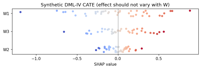
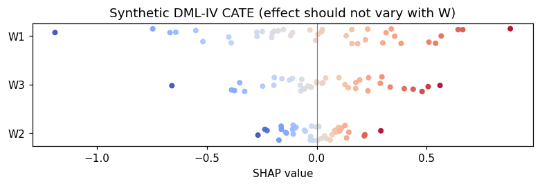
With a constant second stage the only coefficient is \(\hat\theta\). The heterogeneous fit below lets the effect depend on \(W\), which is what SHAP needs. The DGP’s structural effect does not actually vary with \(W\), so those slopes should be small and the average prediction should stay near \(-2\).

Code
het = IVLinearCATE(kind="ridge", n_splits=2, seed=3)
het.fit(W, D, Z, Y, feature_names=["W1", "W2", "W3"])
print("Intercept", round(het.intercept_, 3))
print(pd.DataFrame({"feature": het.feature_names_, "coef": het.feature_coef_}).round(3))
print("Mean predicted CATE", round(float(het.predict(W).mean()), 3))
Intercept -1.791
  feature   coef
0      W1  0.410
1      W2  0.177
2      W3  0.259
Mean predicted CATE -1.779

Summary of Part A

Estimator What it recovers
Naive mean difference Confounded contrast, pulled up by \(C\)
DML-IV Structural effect of the decision, near \(-2\)
PartiallyLinearDML The same confounded contrast, with covariates partialled out of the observed \(W\) only

With binary \(Z\) and \(D\) this is a LATE-style estimand for compliers. A constant second stage collapses it to one number, analogous to cross-fitted 2SLS.

Part B: 401(k) Eligibility and Net Financial Assets

Variable Role in this extract
net_tfa Outcome
e401 Eligibility, the treatment in the partially linear specification
age, inc, fsize, educ, db, marr, twoearn, pira, hown Covariates

Eligibility is the policy variable in the file. The simulation in Part A is where an unobserved confounder and a separate instrument are both present. Part B compares a naive mean difference with PartiallyLinearDML and LinearDML, then explains the linear CATE.

Code
pension = pd.read_csv(data_dir / "data_401k.csv")
x_cols = ["age", "inc", "fsize", "educ", "db", "marr", "twoearn", "pira", "hown"]
Xp = pension[x_cols].to_numpy(dtype=float)
yp = pension["net_tfa"].to_numpy(dtype=float)
dp = pension["e401"].to_numpy(dtype=int)
rng = np.random.default_rng(3141)
train_parts = []
for arm in (0, 1):
    pool = np.flatnonzero(dp == arm)
    train_parts.append(rng.choice(pool, size=int(0.8 * len(pool)), replace=False))
tr = np.concatenate(train_parts)
te = np.setdiff1d(np.arange(len(dp)), tr)
naive_p = float(yp[dp == 1].mean() - yp[dp == 0].mean())
print("Train", len(tr), "Test", len(te), "naive difference", round(naive_p, 1))
Train 7931 Test 1984 naive difference 19559.3

Train–test comparison

Code
results = [{"Estimator": "Naive mean difference", "Learner": "—", "Estimate": naive_p, "Std. err": np.nan}]
for kind, label in (("ridge", "ridge"), ("rf", "rf"), ("gbr", "gbr")):
    model = PartiallyLinearDML(discrete_treatment=True, n_splits=3, model_y=kind, n_estimators=30, random_state=8)
    model.fit(Xp[tr], dp[tr], yp[tr], feature_names=x_cols)
    summary = model.average_treatment_effect()
    results.append({
        "Estimator": "PartiallyLinearDML",
        "Learner": label,
        "Estimate": summary["estimate"],
        "Std. err": summary["std.err"],
    })
result_table = pd.DataFrame(results)
result_table.round(1)
Estimator Learner Estimate Std. err
0 Naive mean difference — 19559.3 NaN
1 PartiallyLinearDML ridge 8478.7 1545.3
2 PartiallyLinearDML rf 8674.2 1525.7
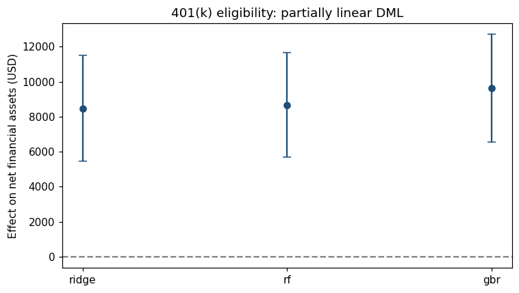
3 PartiallyLinearDML gbr 9637.4 1563.2

Visualize estimates

Code
plot_df = result_table.dropna().reset_index(drop=True)
fig, ax = plt.subplots(figsize=(7.0, 4.0))
ax.errorbar(
    np.arange(len(plot_df)),
    plot_df["Estimate"],
    yerr=1.96 * plot_df["Std. err"],
    fmt="o", color="#1F4E79", capsize=4,
)
ax.axhline(0, color="grey", ls="--")
ax.set_xticks(np.arange(len(plot_df)))
ax.set_xticklabels(plot_df["Learner"])
ax.set_ylabel("Effect on net financial assets (USD)")
ax.set_title("401(k) eligibility: partially linear DML")
fig.tight_layout()

Reading the table. Every PartiallyLinearDML row is the effect of eligibility after partialling out the observed covariates. The naive row is the raw mean difference. There is no simulation truth on this file; stability across learners is the check.

The DML-IV rows from Part A are the right comparison when participation is endogenous and eligibility is only an instrument. That second endogenous regressor is not in data_401k.csv.

SHAP

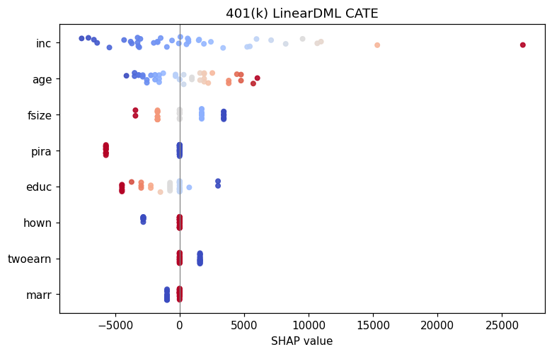
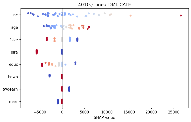
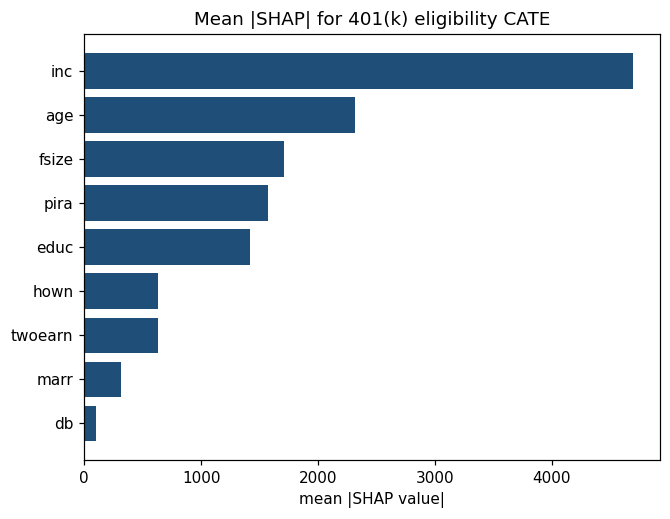
LinearDML supplies \(\hat\tau(X)\) on the training fold. Permutation SHAP uses a subsample of the test fold.

Code
cate_model = LinearDML(discrete_treatment=True, n_splits=2, model_y="rf", n_estimators=30, random_state=9)
cate_model.fit(Xp[tr], dp[tr], yp[tr], feature_names=x_cols)
# Heterogeneous IV surface on the synthetic design, for a side-by-side reading of SHAP.
iv_surface = IVLinearCATE(kind="rf", n_splits=2, seed=4)
iv_surface.fit(W, D, Z, Y, feature_names=["W1", "W2", "W3"])
explanation = explain_cate(
    cate_model, Xp[te], feature_names=x_cols, max_samples=40, n_permutations=6, random_state=9,
)
iv_explanation = explain_cate(
    iv_surface, W, feature_names=["W1", "W2", "W3"], max_samples=40, n_permutations=6, random_state=4,
)
plot_beeswarm(explanation, "401(k) LinearDML CATE")

Code
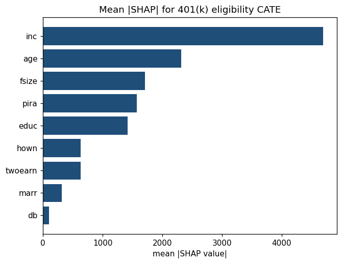
explanation.plot_importance(title="Mean |SHAP| for 401(k) eligibility CATE")

Code
plot_beeswarm(iv_explanation, "Synthetic DML-IV CATE (effect should not vary with W)")

Code
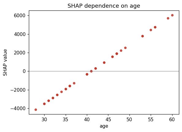
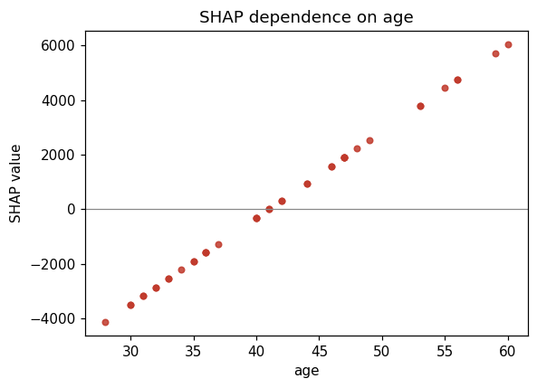
explanation.plot_dependence("age", title="SHAP dependence on age")

Code
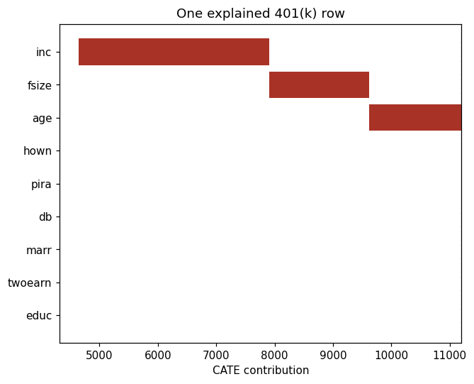
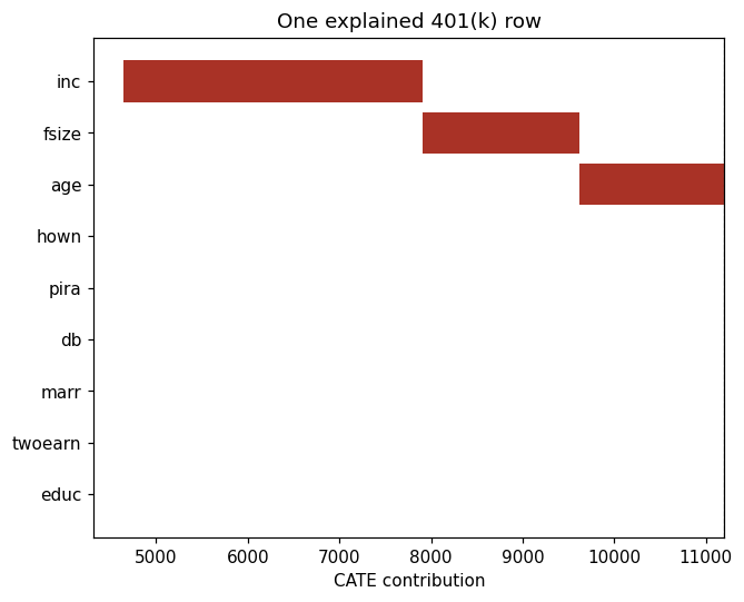
explanation.plot_waterfall(row=0, title="One explained 401(k) row")

Code
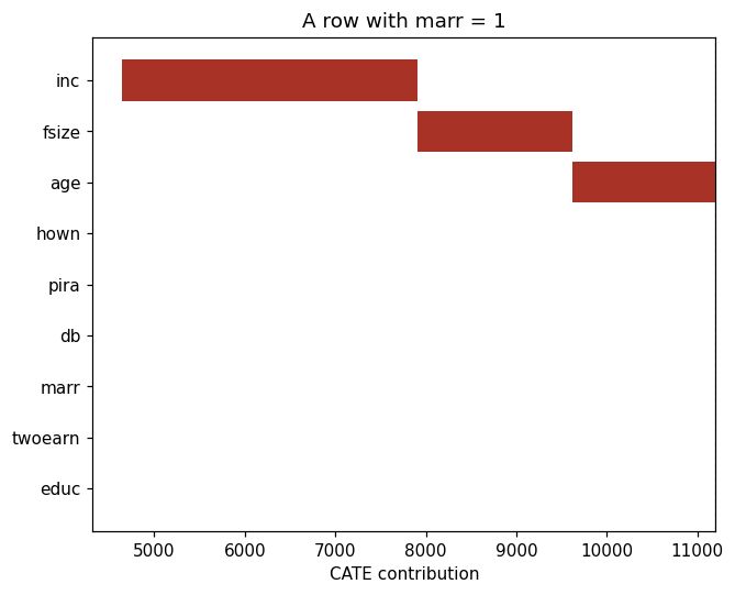
married = explanation.feature_names.index("marr")
hits = np.flatnonzero(explanation.data[:, married] == 1)
row = int(hits[0]) if len(hits) else 0
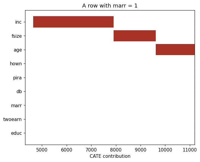
explanation.plot_waterfall(row=row, title="A row with marr = 1")

DML-IV and partially linear CATE surfaces answer different questions. On the simulation they should disagree in level, because only the IV score removes \(C\). On the 401(k) extract the plotted SHAP values describe heterogeneity in the eligibility effect.

Summary

Component Description
IV structure \(Z\) shifts \(D\); \(C\) otherwise confounds \(D\) and \(Y\)
DML-IV Cross-fitted residuals of \(Y\), \(D\), and \(Z\), then \(\tilde Z\) instruments \(\tilde D\)
InstrumentalVariable Linear 2SLS with a bootstrap interval
PartiallyLinearDML No instrument; biased when an unobserved confounder remains
401(k) file Eligibility effect via PartiallyLinearDML and LinearDML
SHAP explain_cate on the linear CATE and on the simulated IV surface

References

  • Chernozhukov, V., et al. (2018). Double/debiased machine learning for treatment and structural parameters. The Econometrics Journal, 21(1), C1–C68.
  • Chernozhukov, V., Hansen, C., & Spindler, M. (2020). DoubleML. Journal of Statistical Software.
  • DoubleML user guide
Back to top