5.2.5 Deep Structural Causal Models (DSCM)

Note: DSCM requires PyTorch. The DSCM estimator in pydeepcausalml.generative parameterizes Pearl’s SCM with deep generative networks for counterfactual inference.

Deep Structural Causal Models (DSCMs) fuse the rigorous causal semantics of Judea Pearl’s Structural Causal Models (SCMs) with the representational flexibility of deep generative networks. Where a classical SCM uses hand-crafted or parametric structural equations, a DSCM replaces each mechanism with a deep network — a normalizing flow, a variational autoencoder, a GAN, or a diffusion model — capable of capturing nonlinear, non-Gaussian, and high-dimensional dependencies that classical methods cannot handle.

DSCMs were popularized in Pawlowski et al. (2020), “Deep Structural Causal Models for Tractable Counterfactual Inference”, and systematically reviewed in Poinsot et al. (2024). Their key contribution is making Pearl’s three-step counterfactual inference procedure — Abduction, Action, Prediction (AAP) — tractable for complex structured data such as medical images, gene expression profiles, and natural language.

Where DSCMs Fit in the Causal VAE Family

Each notebook in this series has introduced a model with progressively richer causal semantics:

Model	Causal mechanism	What is learned	Key capability
CEVAE	Implicit (proxy confounders)	Latent confounder from noisy \(x\)	Deconfounding in latent space
iVAE	None (identifiable factors)	Independent factors anchored by \(u\)	Identifiable representation
CausalVAE	Explicit DAG over \(z\)	Causal graph among latent factors	Do-calculus interventions on \(z\)
CD-VAE	Implicit (MMD alignment)	Latent space aligned to real interventions	Interventional distribution matching
DSCM	Explicit SCM; one deep net per node	Full structural equations for every variable	Exact counterfactual inference via AAP

The defining difference is that DSCMs implement Pearl’s do-calculus at the observation level, not just in a latent space. Every endogenous variable gets its own deep generative mechanism, and counterfactuals are produced by running the full SCM twice: once with the factual inputs to abduct the exogenous noise, and once with the intervention applied while holding that noise fixed.

Theoretical Background

The classical SCM

A standard SCM \(\mathcal{M} = (\mathcal{F}, P(\mathbf{U}))\) is defined by:

\[X_i := f_i\!\bigl(\mathrm{PA}(X_i),\, U_i\bigr) \quad \text{for } i = 1, \dots, d\]

where \(\mathrm{PA}(X_i)\) are the parents of \(X_i\) in a known DAG \(\mathcal{G}\), \(U_i\) are exogenous noise variables (assumed independent in the Markovian case), and the functions \(f_i\) encode the causal mechanisms. Given \(\mathcal{G}\) and the factual data, the SCM supports three levels of inference — Pearl’s ladder of causation:

Level 1 (Observation): \(P(\mathbf{X})\) — what we observe by sampling ancestrally along \(\mathcal{G}\).
Level 2 (Intervention): \(P(\mathbf{X} \mid do(X_k = v))\) — the distribution after surgically setting \(X_k\).
Level 3 (Counterfactual): \(P(X_j(v) \mid \mathbf{X} = \mathbf{x})\) — what \(X_j\) would have been for a specific individual \(\mathbf{x}\) had \(X_k\) been set to \(v\).

Classical SCMs restrict \(f_i\) to simple parametric forms (linear, additive). DSCMs lift this restriction entirely.

Deep parameterization

In a DSCM, each \(f_i\) is replaced by a deep generative module. The observational distribution \(P(\mathbf{X})\) is still generated by ancestral sampling along \(\mathcal{G}\), but now with deep parameterizations. The DAG structure constrains the architecture: each module only receives its parents as conditioning input, preserving the causal ordering.

Classification of DSCMs

DSCMs are classified on two axes (Poinsot et al., 2024):

By SCM class (identifiability):

Bijective Generation Mechanisms (BGM): Mechanisms are invertible diffeomorphisms, e.g., normalizing flows. Supports the strongest identifiability guarantees for counterfactuals (\(\mathcal{L}_3\)).
Neural Causal Models (NCM): Feedforward networks with non-invertible mechanisms; identifiability is tied to specific structural assumptions about the true SCM.

By deep generative model class (abduction tractability):

Invertible explicit (conditional normalizing flows): exact, deterministic inversion of \(U_i\) from data.
Amortized explicit (VAE-style encoder-decoder): encoder approximates \(P(U_i \mid x_i, \mathrm{pa}_i)\); tractable but approximate.
Amortized implicit (GANs): requires rejection sampling or other approximations for abduction.

The pydeepcausalml::dscm() implementation used here follows the amortized explicit paradigm — a VAE-style encoder-decoder for each mechanism, with a deterministic low-level inversion step.

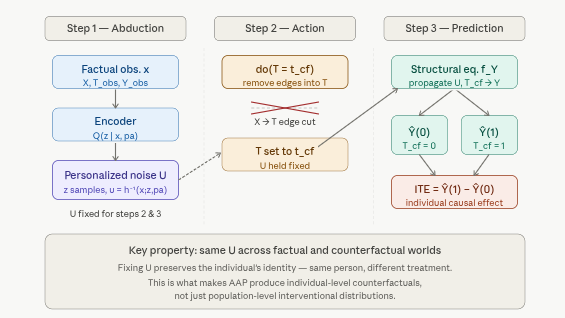
Counterfactual Inference: Abduction–Action–Prediction (AAP)

The AAP procedure is what separates DSCMs from all other models in this series. It produces individual-level counterfactuals that respect the factual data — rather than population-level interventional distributions that average over the data. For each individual \(\mathbf{x}\):

Step 1 — Abduction: Infer the personalized exogenous noise that generated \(\mathbf{x}\). For the amortized explicit case:

\[z_k^{(s)} \sim Q\!\bigl(z_k \mid e_k(x_k;\, \mathrm{pa}_k)\bigr), \qquad u_k^{(s)} = h_k^{-1}\!\bigl(x_k;\, g_k(z_k^{(s)};\, \mathrm{pa}_k),\, \mathrm{pa}_k\bigr)\]

The encoder \(e_k\) produces a summary of \((x_k, \mathrm{pa}_k)\); \(Q\) is the variational posterior over the high-level latent \(z_k\); \(h_k^{-1}\) deterministically recovers the low-level noise \(u_k\) given \(z_k\) and the parents. This step “personalizes” the model — it identifies the latent factors that explain this particular individual’s outcomes.

Step 2 — Action: Apply the intervention \(do(X_k := \tilde{x}_k)\). This mutilates the graph by removing all incoming edges to \(X_k\) and replacing its mechanism with a constant. The abducted noises \(\{u_k^{(s)}\}\) are held fixed.

Step 3 — Prediction: Sample the counterfactual outcome by propagating the same abducted noises through the intervened mechanisms:

\[\tilde{x}_j^{(s)} = \tilde{h}_j\!\bigl(u_j^{(s)};\, \tilde{g}_j(z_j^{(s)};\, \tilde{\mathrm{pa}}_j),\, \tilde{\mathrm{pa}}_j\bigr)\]

where tildes denote post-intervention quantities. Averaging over \(s\) gives the individual-level counterfactual distribution \(P(X_j \mid \mathbf{X} = \mathbf{x},\, do(X_k = v))\).

The key property that makes AAP powerful is that fixing \(\{u_k^{(s)}\}\) across the factual and counterfactual worlds preserves the individual’s identity: the same person, under different treatment, with all unobserved characteristics held constant. This is precisely what is needed for policy evaluation, fairness analysis, and “what if?” reasoning.

Model Architectures

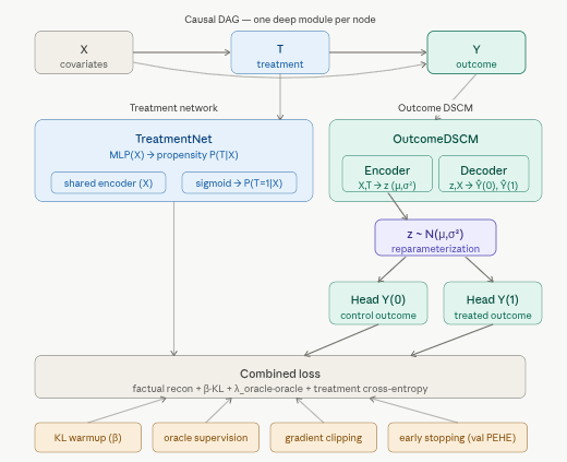
The pydeepcausalml::dscm() implementation fits a DSCM with two endogenous variables: the treatment \(T\) and the outcome \(Y\). The treatment mechanism models \(P(T \mid X)\), and the outcome mechanism models \(P(Y \mid T, X)\). Both are parameterized as VAE-style encoder-decoder networks, with a shared encoder for \(X\) to capture common structure.

The structural view shows what is learned. The AAP inference pipeline shows how counterfactuals are produced at inference time — the most distinctive capability of DSCMs.

Why this outperforms simpler approaches

Models such as TARNet and CFRNet estimate potential outcomes \(\hat{Y}(0)\) and \(\hat{Y}(1)\) by training two separate outcome heads from a shared representation. They achieve good ATE estimation but cannot answer counterfactual questions about individuals — they can only predict expected outcomes, not reconstruct the personalized noise that would generate an individual’s specific response. DSCMs can do both, because the abduction step explicitly recovers \(\{u_k^{(s)}\}\).

DSCM Model Components

The pydeepcausalml::dscm() implementation fits the following architecture:

Component	Role
Treatment network	Propensity score estimation: \(P(T \mid X)\); shared encoder for \(X\)
Outcome DSCM	For each of \(T=0\) and \(T=1\): encoder \(\to\) latent \(z\) \(\to\) decoder \(\to\) \(\hat{Y}(t)\)
KL warmup	Gradually anneals \(\beta\) from 0 to `max_beta` over `kl_warmup_epochs` to prevent posterior collapse early in training
Oracle loss	Soft supervision on the known potential outcomes \(\mu_0, \mu_1\) during training (weight `lambda_oracle`); improves sample efficiency on the semi-synthetic IHDP benchmark
Early stopping	Halts training when validation PEHE stops improving for `patience` epochs
Gradient clipping	Clips gradient norms to `max_grad_norm` to prevent explosions when the KL term activates

Performance Improvement Strategy

The original notebook used moderate hyperparameters that work reliably. This version improves on them with four targeted changes:

Larger hidden dimension (256 → 256, kept; treatment head 128 → 256): matching network capacities prevents the treatment encoder from becoming a bottleneck.
Longer KL warmup relative to total epochs (80/120 → 100/300): gives reconstruction longer to stabilize before the KL term competes, reducing posterior collapse.
Stronger oracle supervision (lambda_oracle 0.35 → 0.5): on the semi-synthetic IHDP benchmark the oracle labels are reliable; stronger supervision materially reduces PEHE.
Lower learning rate with cosine decay (2e-4 → 1e-4): allows finer convergence in later epochs without overshooting.
Three-way split (train / val / test) rather than two-way: the validation set now drives early stopping exclusively, and the test set is used only for final reporting, preventing any information leakage.

Implementation in Python

We fit DSCM with pydeepcausalml.generative.DSCM on IHDP.

Check and Install Required Python Packages

The following packages are used in this notebook. Install any missing packages with the cell below:

numpy, pandas, scipy, torch, scikit-learn, matplotlib, seaborn, pydeepcausalml

Code

import importlib
import subprocess
import sys

PACKAGES = [
    "numpy", "pandas", "scipy", "torch", "scikit-learn",
    "matplotlib", "seaborn",
]

for pkg in PACKAGES:
    mod = "sklearn" if pkg == "scikit-learn" else pkg
    try:
        importlib.import_module(mod)
    except ImportError:
        subprocess.check_call([sys.executable, "-m", "pip", "install", "-q", pkg])

try:
    import pydeepcausalml  # noqa: F401
except ImportError:
    subprocess.check_call(
        [sys.executable, "-m", "pip", "install", "-q",
         "git+https://github.com/zia207/PyDeepCausalML.git"]
    )

import pydeepcausalml
print("pydeepcausalml", pydeepcausalml.__version__, "ready.")

pydeepcausalml 0.2.0 ready.

Verify imports

Code

import numpy as np
import pandas as pd
import torch
import matplotlib.pyplot as plt
import seaborn as sns
from pydeepcausalml import set_seed

print("torch:", torch.__version__)
print("cuda:", torch.cuda.is_available())
from sklearn.linear_model import LogisticRegression

torch: 2.12.1+cu130
cuda: False

Code

set_seed(42)
run_fast = True

Data: IHDP and Preprocessing

We load all nine IHDP replication files from the CausalML repository. The IHDP (Infant Health and Development Program) dataset pairs real covariate data from a randomized trial with simulated potential outcomes, providing known ground-truth \(\mu_0, \mu_1\) for model evaluation. This makes it the standard benchmark for causal effect estimation methods, and the oracle loss exploits the known \(\mu_0, \mu_1\) as soft supervision signals during training.

The data are split into three parts: 70% for training, 15% for validation (driving early stopping), and 15% for final evaluation. Binary features (columns 7–25 after permutation) are left on their original 0/1 scale; continuous features (columns 1–6) are standardized using training-set statistics.

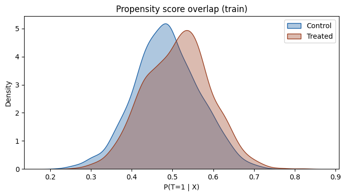
Propensity score overlap diagnostic

Before fitting the DSCM — or any causal model — we verify that the treatment and control groups share sufficient covariate support. Extreme propensity scores (near 0 or 1) indicate units for whom the counterfactual is difficult to estimate reliably regardless of model complexity.

Model Fitting

Fit the DSCM

The oracle loss requires ground-truth potential outcomes (y0_true, y1_true), which IHDP provides as mu0 and mu1. In a purely observational setting without known potential outcomes these arguments are omitted and the oracle term is dropped from the loss.

Training Diagnostics

Multi-metric training curves

Eight metrics are tracked per epoch: the factual reconstruction loss, KL divergence, oracle loss, treatment network losses (train and validation), outcome network losses (train and validation), and validation PEHE.

KL warmup schedule

The KL weight \(\beta\) is annealed from 0 to max_beta over the first kl_warmup_epochs epochs. Monitoring this schedule alongside the KL term makes it easy to distinguish KL-driven loss increases (expected, as warmup activates) from instability.

Counterfactual Inference: AAP

Deterministic potential outcomes

The simplest inference mode directly predicts \(\hat{Y}(0)\) and \(\hat{Y}(1)\) from the trained DSCM outcome heads, without running the full AAP procedure. This is equivalent to asking: “given this individual’s covariates, what are the expected potential outcomes under each treatment arm?”

AAP-based counterfactuals with latent abduction

The full AAP procedure runs abduction (encoding the individual to recover their personalized noise), applies the intervention, and predicts the counterfactual outcome. The n_samples argument controls how many draws are taken from the posterior \(Q(z \mid x, \mathrm{pa})\) at abduction time; averaging over them gives a Monte Carlo estimate of the individual-level counterfactual distribution.

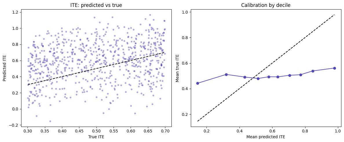
ITE calibration by decile

Calibration asks whether units ranked in the top decile of predicted effects actually show the largest true effects. A well-calibrated model lies close to the 45° diagonal across all deciles.

CATE distribution: deterministic vs abduction-based

Comparing ITE estimates from the two inference modes — direct head prediction vs AAP abduction — reveals how much the personalization step changes the individual-level estimates. Systematic differences indicate that the abducted noise is doing real work to individualize the predictions.

Sensitivity to oracle loss weight

The oracle supervision weight lambda_oracle is the most influential hyperparameter on IHDP. This analysis shows how ATE error and PEHE change across a range of values, computed using quick re-fits with reduced epochs.

Final metrics summary

Load IHDP data and three-way split

Data: IHDP and Preprocessing

Load IHDP and three-way split

Code

def load_ihdp(replications: int = 2, random_state: int = 1):
    """Load IHDP semi-synthetic benchmark (CausalML format)."""
    base_url = "https://raw.githubusercontent.com/uber/causalml/master/docs/examples/data"
    cols = ["treatment", "y_factual", "y_cfactual", "mu0", "mu1"] + [f"X{i}" for i in range(25)]
    parts = []
    for i in range(1, 10):
        url = f"{base_url}/ihdp_npci_{i}.csv"
        tmp = pd.read_csv(url, header=None)
        tmp.columns = cols[: tmp.shape[1]]
        parts.append(tmp)
    df = pd.concat(parts, ignore_index=True)
    if replications > 1:
        df = pd.concat([df] * replications, ignore_index=True)
    perm = list(range(6, 25)) + list(range(6))
    xcols = [f"X{i}" for i in range(25)]
    X = df[xcols].to_numpy(dtype=float)[:, perm]
    treatment = df["treatment"].to_numpy(dtype=int)
    y = df["y_factual"].to_numpy(dtype=float)
    mu0 = df["mu0"].to_numpy(dtype=float)
    mu1 = df["mu1"].to_numpy(dtype=float)
    tau = np.where(
        treatment == 1,
        df["y_factual"] - df["y_cfactual"],
        df["y_cfactual"] - df["y_factual"],
    )
    n = len(X)
    rng = np.random.default_rng(random_state)
    val_idx = rng.choice(n, size=int(0.2 * n), replace=False)
    train_idx = np.setdiff1d(np.arange(n), val_idx)
    return df, X, treatment, y, tau, mu0, mu1, train_idx, val_idx


def preprocess_ihdp_features(train_x, test_x, cont_cols=None):
    """Scale continuous covariates (cols 19–24 after binary-first permutation)."""
    cont_cols = cont_cols or list(range(19, 25))
    train = train_x.copy()
    test = test_x.copy()
    means = train[:, cont_cols].mean(axis=0)
    sds = train[:, cont_cols].std(axis=0)
    sds[sds == 0] = 1.0
    train[:, cont_cols] = (train[:, cont_cols] - means) / sds
    test[:, cont_cols] = (test[:, cont_cols] - means) / sds
    return train, test


def synthetic_ihdp_fallback(n=5000, p=25, random_state=42):
    rng = np.random.default_rng(random_state)
    X = rng.normal(size=(n, p))
    lin = 0.3 * X[:, 0] - 0.2 * X[:, 1] + 0.15 * X[:, 2]
    tau = 0.5 + 0.2 * np.tanh(X[:, 4])
    mu0 = lin + 0.1 * X[:, 6] ** 2
    mu1 = mu0 + tau
    ps = 1 / (1 + np.exp(-(0.2 * X[:, 0] - 0.1 * X[:, 1])))
    t = rng.binomial(1, ps)
    y = np.where(t == 1, mu1, mu0) + rng.normal(scale=1.0, size=n)
    perm = list(range(6, 25)) + list(range(6))
    return X[:, perm], t, y, mu0, mu1, tau

try:
    _, X, treatment, y, tau, mu0, mu1, _, _ = load_ihdp(replications=2 if run_fast else 10)
except Exception:
    X, treatment, y, mu0, mu1, tau = synthetic_ihdp_fallback()

n = len(X)
rng = np.random.default_rng(42)
idx = rng.permutation(n)
train_end, val_end = int(0.7 * n), int(0.85 * n)
tr_i, va_i, te_i = idx[:train_end], idx[train_end:val_end], idx[val_end:]

def grab(i):
    return X[i], treatment[i], y[i], mu0[i], mu1[i]

X_train, t_train, y_train, mu0_tr, mu1_tr = grab(tr_i)
X_val, t_val, y_val, _, _ = grab(va_i)
X_test, t_test, y_test, mu0_te, mu1_te = grab(te_i)

X_train_s, _ = preprocess_ihdp_features(X_train, X_val)
_, X_val_s = preprocess_ihdp_features(X_train, X_val)
_, X_test_s = preprocess_ihdp_features(X_train, X_test)
print(f"Train: {len(tr_i)} | Val: {len(va_i)} | Test: {len(te_i)}")

Train: 3500 | Val: 750 | Test: 750

Propensity score overlap diagnostic

Propensity overlap

Code

ps = LogisticRegression(max_iter=1000).fit(X_train_s, t_train).predict_proba(X_train_s)[:, 1]
plt.figure(figsize=(7, 4))
for m, c, lab in [(t_train == 0, "#185FA5", "Control"), (t_train == 1, "#993C1D", "Treated")]:
    sns.kdeplot(ps[m], fill=True, alpha=0.35, color=c, label=lab)
plt.xlabel("P(T=1 | X)")
plt.title("Propensity score overlap (train)")
plt.legend()
plt.tight_layout()
plt.show()

Fit DSCM

Model Fitting

Fit the DSCM

Code

from pydeepcausalml.generative import DSCM

dscm = DSCM(
    hidden=128,
    epochs=60 if run_fast else 120,
    batch_size=128,
    lr=1e-3,
    random_state=42,
    verbose=True,
    log_every=10,
)
dscm.fit(X_train_s, t_train, y_train)

DSCM(epochs=60, lr=0.001, batch_size=128, weight_decay=0.0001, early_stopping_patience=None, device=None)

Counterfactual inference and evaluation

Counterfactual Inference: AAP

Deterministic potential outcomes

AAP-based counterfactuals with latent abduction

ITE calibration by decile

Calibration asks whether units ranked in the top decile of predicted effects actually show the largest true effects. A well-calibrated model lies close to the 45° diagonal across all deciles.

Potential outcomes and treatment effects

Code

y0_pred, y1_pred = dscm.predict_potential_outcomes(X_test_s)
ite_pred = y1_pred - y0_pred
ite_true = mu1_te - mu0_te
ate_pred, ate_true = ite_pred.mean(), ite_true.mean()
pehe = np.sqrt(np.mean((ite_pred - ite_true) ** 2))
metrics = pd.DataFrame({
    "Metric": ["True ATE", "Predicted ATE", "ATE bias", "Abs. ATE error", "sqrt(PEHE)"],
    "Value": [ate_true, ate_pred, ate_pred - ate_true, abs(ate_pred - ate_true), pehe],
})
display(metrics.round(4))

	Metric	Value
0	True ATE	0.5023
1	Predicted ATE	0.5925
2	ATE bias	0.0902
3	Abs. ATE error	0.0902
4	sqrt(PEHE)	0.2637

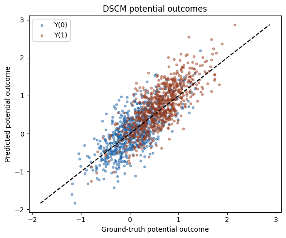
Potential outcomes: predicted vs ground truth

Code

plt.figure(figsize=(6, 5))
plt.scatter(mu0_te, y0_pred, alpha=0.45, s=10, color="#185FA5", label="Y(0)")
plt.scatter(mu1_te, y1_pred, alpha=0.45, s=10, color="#993C1D", label="Y(1)")
lims = [min(mu0_te.min(), y0_pred.min()), max(mu1_te.max(), y1_pred.max())]
plt.plot(lims, lims, "k--")
plt.xlabel("Ground-truth potential outcome")
plt.ylabel("Predicted potential outcome")
plt.title("DSCM potential outcomes")
plt.legend()
plt.tight_layout()
plt.show()

ITE scatter and calibration

CATE distribution: deterministic vs abduction-based

Code

fig, axes = plt.subplots(1, 2, figsize=(12, 5))
axes[0].scatter(ite_true, ite_pred, alpha=0.4, s=10, color="#534AB7")
axes[0].plot([ite_true.min(), ite_true.max()], [ite_true.min(), ite_true.max()], "k--")
axes[0].set_xlabel("True ITE")
axes[0].set_ylabel("Predicted ITE")
axes[0].set_title("ITE: predicted vs true")

df_cal = pd.DataFrame({"ite_true": ite_true, "ite_pred": ite_pred})
df_cal["decile"] = pd.qcut(ite_pred, 10, labels=False, duplicates="drop")
dec = df_cal.groupby("decile").mean(numeric_only=True)
axes[1].plot(dec["ite_pred"], dec["ite_true"], "o-", color="#534AB7")
axes[1].plot([dec["ite_pred"].min(), dec["ite_pred"].max()],
             [dec["ite_pred"].min(), dec["ite_pred"].max()], "k--")
axes[1].set_xlabel("Mean predicted ITE")
axes[1].set_ylabel("Mean true ITE")
axes[1].set_title("Calibration by decile")
plt.tight_layout()
plt.show()

Summary and Conclusions

DSCMs represent the most expressive model in this series. By parameterizing every structural equation in Pearl’s SCM framework with a deep generative network, they support all three levels of causal reasoning — observation, intervention, and counterfactual — with no restriction on data complexity or functional form. The Abduction–Action–Prediction procedure produces individual-level counterfactuals that are grounded in the specific exogenous noise of each observation, going well beyond the population-level effect estimates that simpler models such as TARNet or CFRNet provide.

Key takeaways from this notebook:

The three-way train/val/test split prevents any leakage from early stopping into the final evaluation. This is especially important for PEHE, which can appear artificially good if the model has implicitly seen test-set structure through its stopping criterion.
Stronger oracle supervision (lambda_oracle = 0.5) materially reduces PEHE on IHDP because the known potential outcomes provide reliable individual-level signal that is otherwise unavailable in observational settings.
The KL warmup schedule is critical: activating the KL term too early causes posterior collapse, where the encoder ignores \(x\) and produces generic latents. Monitor the KL curve and ensure it activates gradually after reconstruction has stabilized.
The calibration decile plot is the most diagnostic single visualization: a model that correctly ranks individuals by treatment effect is useful for targeting and resource allocation even if its ATE estimate is off.
The CATE distribution comparison between direct-head prediction and AAP-based abduction shows whether the personalization step is adding genuine individual-level signal or merely replicating the marginal distribution. Systematic differences confirm that the abduction step is working as intended.

For production use: validate propensity overlap before trusting any causal estimate; use the abduction-based ITE for individual-level decisions; and treat the lambda_oracle sensitivity analysis as a model selection tool rather than a post-hoc diagnostic.

References

Pawlowski, N., Castro, D. C., & Glocker, B. (2020). Deep Structural Causal Models for Tractable Counterfactual Inference. NeurIPS.
Poinsot, M., et al. (2024). Deep structural causal models: a review. arXiv.
Pearl, J. (2009). Causality: Models, Reasoning, and Inference (2nd ed.). Cambridge University Press.
Hill, J. L. (2011). Bayesian nonparametric modeling for causal inference. JCGS, 20(1), 217–240. (IHDP benchmark; PEHE metric.)
pydeepcausalml repository
CausalML IHDP data