Python Banner

4. Double/Debiased Machine Learning

Two powerful methodologies have historically talked past each other:

Machine learning predicts outcomes with remarkable accuracy, but its regularization techniques — shrinking or zeroing out coefficients to prevent overfitting — introduce systematic bias into any coefficient it produces. You can’t use a Lasso regression to estimate a causal effect and trust the result.

Classical econometrics (OLS, IV, etc.) produces unbiased, inferentially valid estimates, but breaks down under high dimensionality. With hundreds or thousands of control variables, standard regression is either infeasible or hopelessly overfit.

Double Machine Learning solves both problems simultaneously. It uses ML’s predictive power to handle high-dimensional confounders, then recovers valid causal inference through a clever two-step residualization procedure.

How it works

The model

DML assumes a partially linear data-generating process:

\[ \begin{align} Y &= \theta D + g(X) + \varepsilon \\ D &= m(X) + V \end{align} \]

where \(Y\) is the outcome, \(D\) is the treatment, \(X\) is a (potentially very large) vector of confounders, and \(\theta\) is the causal effect you want. The functions \(g(X)\) and \(m(X)\) are called nuisance functions — they govern how confounders affect the outcome and treatment, but you don’t care about them directly.

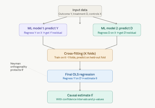
The five-step pipeline

Step 1 — Residualize the outcome. Train any ML model to predict \(Y\) from \(X\). Compute the residual \(\tilde{Y} = Y - \hat{g}(X)\): the part of \(Y\) that confounders cannot explain.

Step 2 — Residualize the treatment. Train a second ML model to predict \(D\) from \(X\). Compute \(\tilde{D} = D - \hat{m}(X)\): the part of \(D\) that confounders cannot explain.

Step 3 — Cross-fit to prevent overfitting. If you train the nuisance models and compute residuals on the same data, the residuals will be artificially small (overfitting). Instead, split the data into \(K\) folds, train on \(K-1\) folds, and predict residuals on the held-out fold. Rotate through all folds and aggregate.

Step 4 — Final OLS. Regress \(\tilde{Y}\) on \(\tilde{D}\): \[\tilde{Y} = \theta\,\tilde{D} + \varepsilon\]

The coefficient \(\hat{\theta}\) is your causal estimate. By construction, you’ve partialled out all confounding variation captured in \(X\).

Step 5 — Inference. Because of the orthogonality property (below), \(\hat{\theta}\) is \(\sqrt{n}\)-consistent and asymptotically normal, giving you valid standard errors, confidence intervals, and p-values.

Double ML flowchart

Why this works: Neyman orthogonality

The critical insight is that the score function used to estimate \(\theta\) is orthogonal to the nuisance parameters. In plain terms: if your ML models for \(g(X)\) and \(m(X)\) are slightly wrong — which they always are — those errors have only a second-order (negligible) impact on \(\hat{\theta}\). This is the “debiasing” step that makes valid inference possible despite using regularized ML.

Supported models and causal structures

PyCausalML is learner-agnostic for the nuisance stages — you can plug in virtually any supervised learning algorithm:

Category	Examples
Penalized linear	Lasso, Ridge, Elastic Net
Tree-based	Random Forest, gradient boosting, XGBoost
Neural networks	MLPs via scikit-learn
Other	SVM, k-NN

The notebooks in this chapter use these structural models:

Model	When to use	PyCausalML estimator
PLR — Partially Linear Regression	Standard observational setting; a constant effect	PartiallyLinearDML
Linear / sparse CATE	The effect varies linearly (or sparsely) with covariates	LinearDML, SparseLinearDML
IRM — Interactive Regression Model	Binary treatment; doubly robust score for the ATE and a flexible CATE	InteractiveRegressionDML
PLIV — Partially Linear IV	Endogenous treatment; a valid instrument	Cross-fitted residual-on-residual IV, plus InstrumentalVariable
Nonparametric CATE	A flexible final stage on the orthogonal pseudo-outcome	NonParamDML, CausalForestDML, KernelDML

Advantages

Capability	What it enables
High dimensionality	Works when the number of controls \(p \gg n\)
Nonlinearity	Captures complex confounder–outcome relationships OLS cannot
Valid inference	Produces standard errors, CIs, and hypothesis tests
Robustness	Resilient to moderate ML estimation error (orthogonality)
Modularity	Swap learners freely; gradient boosting today, random forests tomorrow

Limitations

No hidden confounders. Like all observational methods, standard DML (PLR) assumes unconfoundedness: every variable affecting both \(D\) and \(Y\) is in \(X\). An unmeasured confounder still biases \(\hat{\theta}\). The PLIV variant handles endogeneity, but requires valid instruments.

Sample size still matters. DML handles high dimensionality but not small n. The final regression step requires enough observations for asymptotic normality to hold.

Nuisance functions remain black boxes. \(\hat{\theta}\) is interpretable; \(\hat{g}(X)\) and \(\hat{m}(X)\) are not. You learn the effect of treatment but not how each confounder influences the outcome.

Computational cost. Cross-fitting means training \(K\) nuisance models per variable instead of one. Expect runtime roughly \(K\times\) that of a comparable OLS workflow.

Weak instruments. If you use PLIV, DML inherits the weak-instrument problem from classical 2SLS — a weak instrument inflates standard errors and can bias estimates.

Python ecosystem

Primary package: PyCausalML

The estimators in this chapter live in pycausalml.double_machine_learning.

• Partially linear and interactive models: PartiallyLinearDML, InteractiveRegressionDML
• Heterogeneous effects: LinearDML, SparseLinearDML, NonParamDML, CausalForestDML, KernelDML
• Cross-fitted first stages for every estimator
• Influence-function standard errors and confidence intervals on the average effect
• SHAP explanations of a fitted CATE through explain and pycausalml.interpretation

Nuisance learners are scikit-learn models (random forests, gradient boosting, ridge, lasso). Later notebooks also show pipelines, averaged ensembles, and a small hyperparameter grid around the same orthogonal score.

A related estimator: causal forests

If the question is who benefits from treatment rather than a single average effect, CausalForest (honest trees) and CausalForestDML (a forest on the doubly robust pseudo-outcome) are the natural next tools. They use a related but distinct splitting criterion and are built for effect heterogeneity.

Applications

DML is the natural choice wherever causal questions meet high-dimensional data:

• Economics — price elasticity controlling for thousands of product and market characteristics
• Marketing — true ad-campaign lift after controlling for browsing history and demographics
• Healthcare — drug efficacy controlling for genomic or electronic health record data
• Policy evaluation — job-training program impact controlling for employment history, education, and local conditions

Double Machine Learning is a state-of-the-art method for estimating causal effects when confounders are high-dimensional. It lets you use the predictive power of random forests, gradient boosting, or penalized regression to control for confounders, without giving up the standard errors required to make a causal claim. PyCausalML implements that workflow for partially linear, interactive, instrumental-variable, panel, and clustered designs. Like any observational method, it still relies on the design assumptions of the model you choose.

Resources

Key References

• Chernozhukov, V., Chetverikov, D., Demirer, M., Duflo, E., Hansen, C., Newey, W., & Robins, J. (2018). Double/debiased machine learning for treatment and structural parameters. The Econometrics Journal, 21(1), C1–C68.
• Chernozhukov, V., Hansen, C., & Spindler, M. (2020). DoubleML – Double/debiased machine learning in R and Python. Journal of Statistical Software.

Documentation

• DoubleML user guide — the method, independent of this package
• PyCausalML double_machine_learning module: PartiallyLinearDML, LinearDML, SparseLinearDML, NonParamDML, CausalForestDML, KernelDML, InteractiveRegressionDML